Question 1: What is orthogonal downconversion?
The goal of downconversion is to shift the spectrum of high-frequency signals (such as RF or IF signals) to lower frequencies for subsequent processing.
For example: In the environment, there areA, B, C, D…vehicles. Imagine this scenario: the apocalypse is coming, and there is only one road that will not collapse, but only one vehicle is allowed to stop there. We call this point“frequency point.” Each vehicle carries survival supplies, and we now move vehicle A from its original position to the 0 “frequency point.” Clearly, during the moving process, the “information (supplies)” carried by the vehicle will not be lost. When the apocalypse arrives, everything around will collapse, leaving only vehicle A at the 0 “frequency point” (vehicle A is just a carrier; the focus is on the information it carries). We name this apocalypse “low-frequency filtering.”
Let’s derive the relevant formulas for “frequency shifting”:
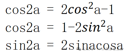
Triangle transformation formula:
Frequency shifting formula (mixing):
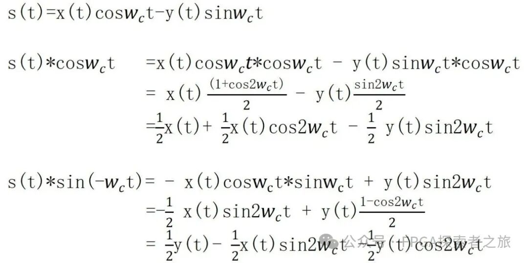
At this point, we have a basic understanding of frequency shifting. Now we will begin to shift the original frequency point to the 0 “frequency point,” as illustrated below:
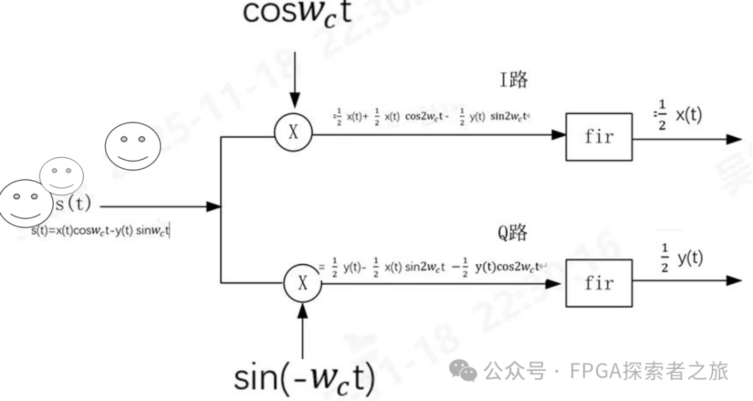
Figure 1. Schematic diagram of orthogonal downconversion
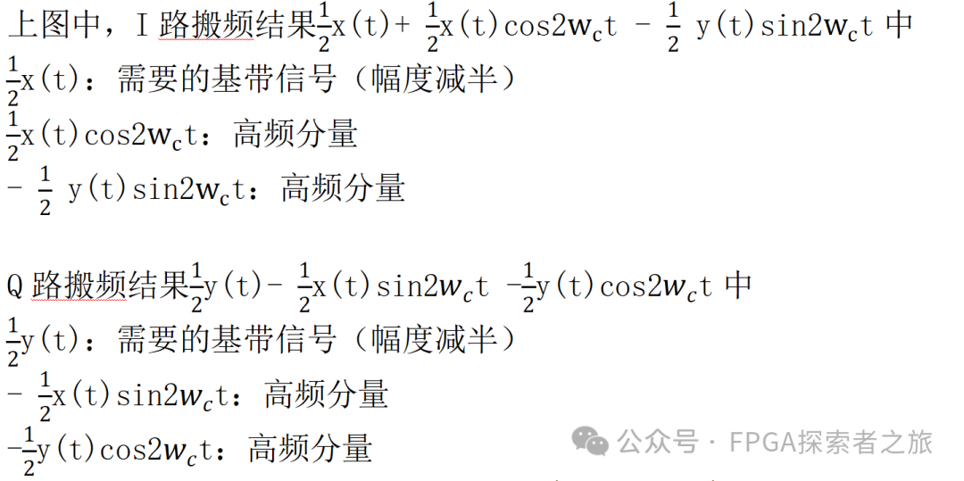
Therefore, after passing through the FIR low-pass filter: onlyx(t) and –y(t) components remain. Then we can proceed with subsequent processing!
Summary: Orthogonal downconversion can be summarized as frequency shifting + low-pass filtering
Advantages of orthogonal downconversion: Ordinary downconversion loses the phase information of the signal. In contrast, orthogonal downconversion retains all information of the signal (including amplitude and phase) intact. In Figure 1, we use two parallel downconversion processes.
Orthogonal downconversion structure: It uses two local oscillator signals, which have the same frequency but are 90 degrees out of phase.
The mathematical core is to use a complex local oscillator signal:
Local oscillator signal= cos(2πft) – j * sin(2πft)
Multiply this complex local oscillator with the input signal (mixing):
I path = Input signal × cos(2πft)
Q path = Input signal × -sin(2πft)
This process ultimately yields baseband I/Q signals.
Processing steps:
1. The input high-frequency signal is simultaneously sent to the I path and Q path.
2. The I path signal is multiplied by cos(2πft)
The Q path signal is multiplied by -sin(2πft)
3. The outputs of the two multipliers pass through low-pass filters to remove high-frequency components, ultimately yielding two low-frequency signals: I(t) and Q(t).
Final output: The output of orthogonal downconversion is not a single real signal, but a complex signal, which can be expressed as:
s_out(t) = I(t) + j * Q(t)
This complex signal contains all the information of the original signal (amplitude and phase).
Question 2: Why use orthogonal downconversion during ADC sampling processing?
1. Satisfy the Nyquist sampling theorem and reduce the requirements for ADC sampling rate
For real signals: According to the Nyquist sampling theorem, the sampling frequencyfs must be greater than twice the highest frequency of the signal to recover the signal without aliasing. If an RF signal has a carrier frequency of fc and a bandwidth of B, then directly sampling it requires a sampling rate fs > 2(fc + B/2), which can be very high and places extreme demands on the performance and cost of the ADC.
For complex signals (after orthogonal downconversion): After orthogonal downconversion, we shift the signal’s spectrum from the center frequencyfc to zero intermediate frequency. At this point, the signal’s spectrum range is -B/2 to +B/2. For this zero intermediate frequency complex signal, its positive and negative spectra are asymmetric and contain different information. Theoretically, it only requires a sampling rate fs > B (the bandwidth of the signal) to sample without aliasing.
Conclusion: By using orthogonal downconversion to convert the signal into a baseband complex signal, the requiredADC sampling rate is significantly reduced from > 2fc to > B, greatly lowering the performance requirements for ADC devices and reducing the computational burden for subsequent data processing.
2. Retain complete phase information, facilitating demodulation of modulated signals
Communication systems (such as QPSK, 16QAM, 5G, etc.) commonly use complex modulation methods that modulate both amplitude and phase.
If only one downconversion (real signal) is used, we can only obtain information projected onto one axis, making it impossible to distinguish whether the phase is +90 degrees or -90 degrees; however, if we use orthogonal downconversion (I/Q paths), we obtain a vector on a complex plane. The length of this vector represents the amplitude, and the angle with the I axis represents the phase. This way, we can unambiguously demodulate the original transmitted symbols.
In summary, using orthogonal downconversion before ADC sampling aims to efficiently and losslessly convert high-frequency communication signals into baseband complex signals that can be processed at lower sampling rates, thereby ensuring the integrity of the information while significantly reducing the system’s requirements for ADC performance and subsequent processing resources.