Radar waveforms can be classified into pulse signals and continuous wave signals based on the radar system, and further categorized by modulation methods.
-
Pulse Signals
-
Single Carrier Frequency
-
Intra-Pulse, Inter-Pulse, or Pulse Group Coding
-
Coherent Pulse Train
Continuous Wave Signals
-
FM-CW
-
FSK-CW
-
LFM+FSK
-
SF-CW
-
FM+SFCW
Today, we will focus on the FMCW waveform.
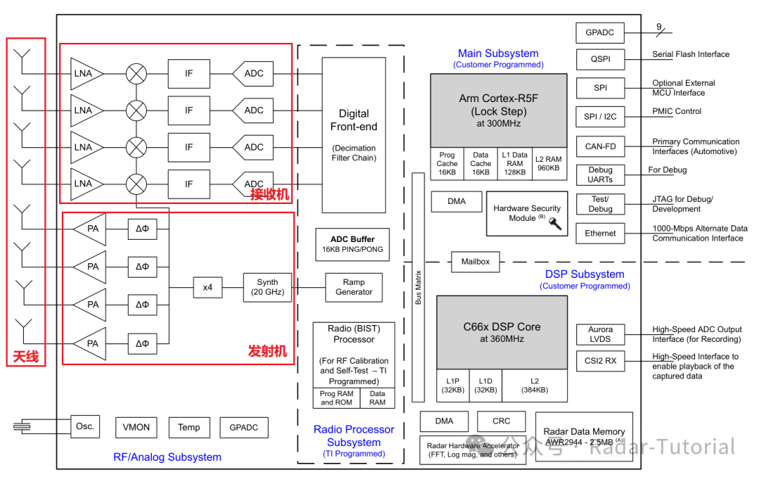
The derivation of the signal model requires a clear understanding of the radar signal transmission-reception model, which provides a general overview of the radar system’s components. The diagram below is from the TI AWR2944 Functional Block Diagram, which is roughly divided into antenna, transmitter, receiver, and signal processor.
-
After generating the modulated radar signal, it is up-converted and amplified before being radiated into space from the transmitting antenna;
-
When the electromagnetic wave encounters a target, scattering occurs, and the backscattered electromagnetic wave is received by the radar receiving antenna;
-
The transmitted and received signals produce a beat frequency signal after passing through a mixer, and a series of signal processing steps are performed on this signal to extract effective information about the target, such as distance, speed, and angle.
Expression for the transmitted signal

-
f0: Starting frequency
-
K: Modulation slope, K=B/T
Expression for the received signal, which is the delayed version of the transmitted signal

-
Ar: Amplitude of the received signal
-
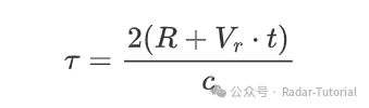
τ: Delay of the echo signal, assuming a target is located at distance R, with a constant speed Vr, the corresponding delay is
-
R: Distance to the target
-
Vr: Radial speed of the target
-
c: Speed of light
Expression for the beat frequency signal, obtained by mixing the transmitted and received signals and passing through a low-pass filter

Since τ/T<<1, the last term can be ignored. Substituting τ into the above expression and rearranging gives the following expression

Since Vr<<c, the last term can be ignored

For convenience in subsequent discussions, we set the amplitude to 1. To measure the target’s speed, a series of chirp signals need to be transmitted. Assuming a total of L chirps are transmitted,

-
L: Number of chirps in one frame, l: Index of the chirp
-
Tc: Chirp period
The distance change caused by the target’s motion corresponds to a frequency much smaller than the frequency corresponding to the target distance (Vr·Tc·L<<R), thus we assume that the target does not move more than one distance bin within a frame. This assumption may not hold for high-speed moving targets.

Where
-
fr=2KR/c: Frequency corresponding to the distance
-
fd=2Vr/λ: Doppler frequency
Based on the above expressions, we will simulate the echo signal using MATLAB. The code is as follows:
close all;clear;
f0=77e9;c=physconst('LightSpeed');lambda = c/f0;B = 600e6;Tc = 40e-6;K = B/Tc;fs=20e6;ts = 1/fs;N = 1024;L = 64;dt = (0:N-1)*ts;
R = 20;V = 10;fr = K*2*R/c;fd = 2*V/lambda;
% beat signal
gereratesig = zeros(N,L);for i = 1:L    sig(:,i) = cos(2*pi*((fr+fd)*dt + fd*Tc*i + 2*f0*R/c));end
% 2d-fft
rangeWin = repmat(hann(N), 1,L);dopplerWin = repmat(hann(L)',N/2,1);
rangeFFTWin = fft(sig.*rangeWin, N, 1);dopFFTWin = fft(rangeFFTWin(1:N/2,:).*dopplerWin, L, 2);
figure;subplot(121);mesh(abs(rangeFFTWin(1:N/2,:)));title('rangeFFT');xlabel('dopBins');ylabel('rangeBins');view([1 0 0])subplot(122);mesh(abs(dopFFTWin));title('dopplerFFT');xlabel('dopBins');ylabel('rangeBins');view([0 0 1])
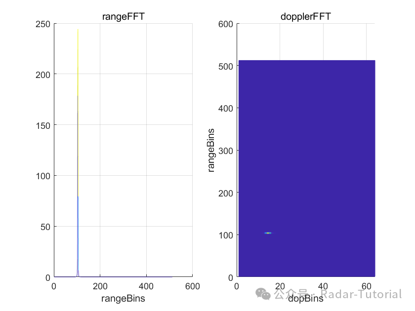
The results after executing the 2D FFT are as follows:
This concludes today’s content sharing. I hope it is helpful to everyone. Feel free to like, comment, and share. See you in the next article!