
The state equation and observation equation are both two-dimensional and nonlinear. There are Chinese comments, and you can modify the code as needed.
<span>After subscribing to the column, you can directly view the source code, paste it into a MATLAB empty script, and run it to obtain results.</span>
Article Directory
- Program Introduction
- Running Results
- MATLAB Source Code
Program Introduction
Overview of Program FunctionalityThis program demonstrates the CKF (Cubature Kalman Filter) state estimation process on a two-dimensional nonlinear system. By constructing the true trajectory of the nonlinear system and adding process/observation noise to generate observation data, the CKF is used for estimation, and the results are compared with the unfiltered results. Finally, error curves, error distribution (CDF), and numerical statistics (maximum, mean, standard deviation) are provided.
Model and Data
- The state is two-dimensional, containing nonlinear driving terms and constant speed growth terms;
- The observations are two nonlinear quantities: one dimension is a square term, and the other dimension is a cubic term;
- Both process noise and observation noise are zero-mean Gaussian, with covariance adjustable by
<span>Q</span>and<span>R</span>; - The program fixes the random seed to ensure reproducibility.
Plotting and Output
- Draw a two-dimensional trajectory comparison chart (true/unfiltered/CKF);
- Plot state curves and error curves for each dimension;
- Draw the CDF of the error to visually compare filtering effects;
- Output the maximum, mean, and standard deviation of errors for each dimension in the command line.
Parameters and Usage Recommendations
- Increase
<span>Q</span>: The filter is more sensitive to model uncertainty, tracking changes faster but with more noise; - Increase
<span>R</span>: Less trust in measurements, resulting in smoother results but potentially lagging; - Time length, nonlinear intensity, and noise level can be treated as experimental variables to observe the robustness and convergence behavior of the CKF.
Applicability and Extensions
- Suitable for demonstrating the idea of derivative-free filtering in the “nonlinear + Gaussian noise” scenario;
- State/observation functions can be smoothly replaced to adapt to tasks such as target tracking and navigation;
- Easy to extend to higher dimensions, different noise levels, and comparative experiments with varying nonlinear intensities.
Running Results
The figures plotted with the X and Y axes include comparison images before and after filtering: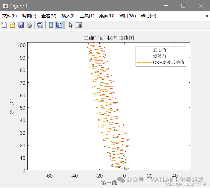 State curves for each axis:
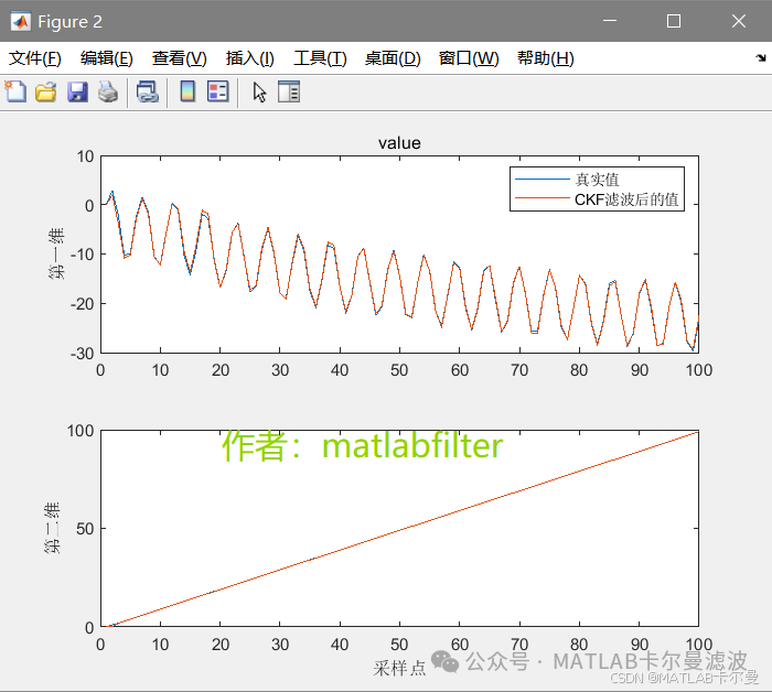
MATLAB Source Code
Part of the code is as follows:
% CKF's two-dimensional filtering program example
% Author contact: VX:matlabfilter (for paid consultation unless previously agreed)
% 2025-08-28/Ver1
clear;clc;close all;% Clear workspace, command line, close small windows
rng(0);% Fix random seed
%% Filter model initialization
t =1:1:100;% Define time series
Q =0.1*diag([1,1]);% Set process noise covariance matrix
w =sqrt(Q)*randn(size(Q,1),length(t));% Generate
% Observation noise covariance matrix and observation noise
R =1*diag([1,1]);
v =sqrt(R)*randn(size(R,1),length(t));
% Initial state estimate covariance matrix
P0 =1*eye(2);
% Initialize state vector
X =zeros(2,length(t));% Allocate space for true state values
Z=zeros(2,length(t));% Define observation values (allocate space)
Z(:,1)=[X(1,1)^2/20;X(2,1)^3]+v(:,1);% Observations
%% Motion model
X_=zeros(2,length(t));% Allocate space for unfiltered state
X_(:,1)=X(:,1);% Assign initial value to unfiltered state
Download link for the complete code:
https://mall.bilibili.com/neul-next/detailuniversal/detail.html?isMerchant=1&page=detailuniversal_detail&saleType=10&itemsId=13019277&loadingShow=1&noTitleBar=1&msource=merchant_share
Or click “Read the original text” at the end of the article to jump.
<span>If you need help or have custom code requirements related to navigation and positioning filtering, please contact the author via WeChat below.</span>