Basic Fitting Preparation
The basic fitting user interface sorts the data in ascending order before fitting. If the dataset is large and the values are not sorted in ascending order, the basic fitting user interface may take a long time to preprocess the data before fitting.
This article is adapted from the MATLAB help center, for detailed content see:
https://ww2.mathworks.cn/help/matlab/data_analysis/interactive-fitting.htmlSorting the data in advance can speed up the processing time of the basic fitting user interface. To create sorted vectors x_sorted and y_sorted from the data vectors x and y, use the MATLAB sort function:
[x_sorted, i] = sort(x);y_sorted = y(i);Opening the Basic Fitting User Interface
To use the basic fitting user interface, you must first plot the data in the figure window using any MATLAB plotting command that generates only x and y data. To open the basic fitting user interface, select Tools > Basic Fitting from the top menu of the figure window.
Example: Using the Basic Fitting User Interface
This example demonstrates how to fit, visualize, analyze, save polynomial regression, and generate code using the basic fitting user interface.
Loading and Plotting Census Data
The file census.mat contains U.S. population data from 1790 to 1990 at 10-year intervals. To load and plot the data, type the following commands at the MATLAB prompt:
load censusplot(cdate,pop,'ro')The load command adds the following variables to the MATLAB workspace: cdate – a column vector containing the years from 1790 to 1990 (in increments of 10). It is the predictor variable. pop – a column vector of the U.S. population for each year in cdate. It is the response variable. The data vectors are sorted in ascending order by year. The plot shows the population as a function of the year. Now, the data is ready for equation fitting to establish a model of population growth over time.
Predicting Census Data with a Cubic Polynomial Fit
-
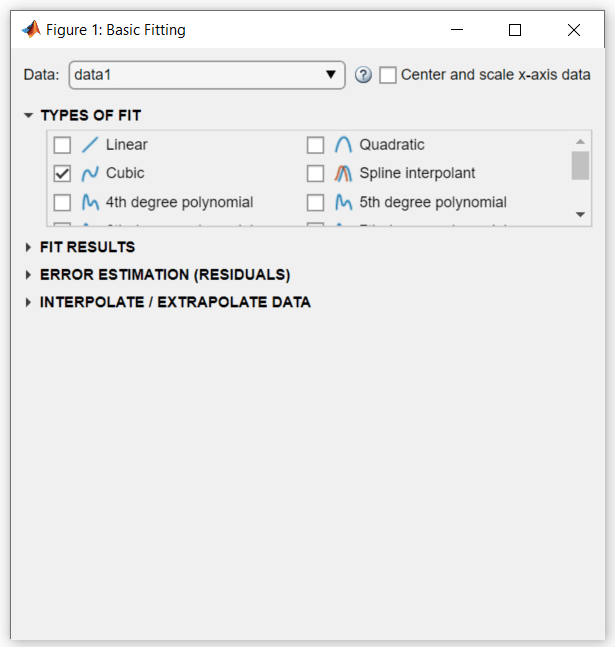
Select Tools > Basic Fitting in the figure window to open the “Basic Fitting” dialog.
-
In the Type of Fit area of the “Basic Fitting” dialog, check the Cubic checkbox to fit the data with a cubic polynomial.
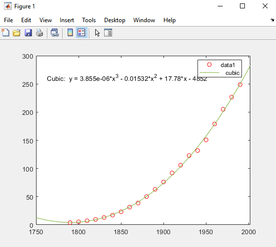
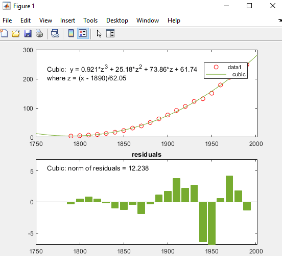
MATLAB fits the data according to the options and adds the cubic regression line to the plot, as shown below.
While calculating the fit, MATLAB encountered a problem and issued the following warning:
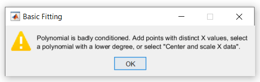
This warning indicates that the coefficients of the computed model are sensitive to the random errors in the response (measured population). It also provides some suggestions to help improve the fit.
-
Continue with the cubic fit. Since new observations cannot be added to the census data, you can improve the fit by converting the available values to Z-scores before recalculating the fit. Check the Center and Scale x-axis Data checkbox in the upper right corner of the dialog to have the basic fitting tool perform the transformation.
Under Error Estimation (Residuals), check the Residual Norm checkbox. Select Bar Graph as the Plot Style.
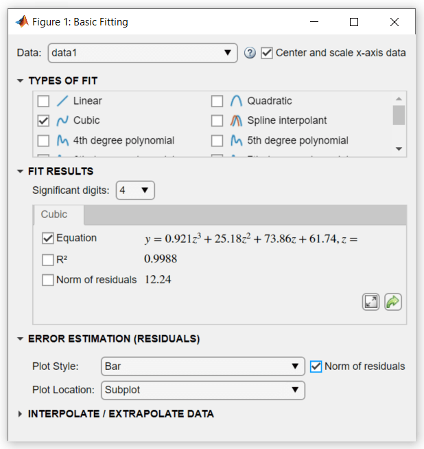
After selecting these options, a residual subplot will be created as a bar graph.
(Source: Mathematical Modeling BOOM)