What is Signal Processing?
Signal processing is the discipline of performing various operations and analyses on signals with the aim of extracting, enhancing, or storing useful information within the signals. Signals can take various forms of data, such as sound, images, and biological electrical signals.
Classification of Signals
-
Continuous Signals: Signals that vary continuously over time
-
Discrete Signals: Signals sampled at specific time points
-
Analog Signals: Signals with continuously varying amplitudes
-
Digital Signals: Signals with quantized amplitudes
Core Concept: Fourier Transform
The Fourier Transform is one of the most important mathematical tools in signal processing, allowing us to convert signals from the time domain (temporal dimension) to the frequency domain (frequency dimension), enabling us to analyze the various frequency components contained within the signals.
Python Implementation: Signal Generation and Processing
1. Generating Composite Signals
import numpy as np
import matplotlib.pyplot as plt
from scipy import signal
# Set style
plt.style.use('seaborn-v0_8-whitegrid')
plt.rcParams['font.sans-serif'] = ['SimHei']
plt.rcParams['axes.unicode_minus'] = False
# Generate signal
def generate_signal(duration=1.0, sample_rate=1000):
    """
    Generate a composite signal containing multiple frequency components
    """
    t = np.linspace(0, duration, int(sample_rate * duration), endpoint=False)
    # Generate three sine waves of different frequencies
    freq1 = 5   # 5 Hz
    freq2 = 20  # 20 Hz
    freq3 = 50  # 50 Hz
    signal1 = np.sin(2 * np.pi * freq1 * t)
    signal2 = 0.5 * np.sin(2 * np.pi * freq2 * t)
    signal3 = 0.3 * np.sin(2 * np.pi * freq3 * t)
    # Combine signals and add noise
    clean_signal = signal1 + signal2 + signal3
    noisy_signal = clean_signal + 0.2 * np.random.normal(size=clean_signal.shape)
    return t, clean_signal, noisy_signal
# Plot signals
t, clean_signal, noisy_signal = generate_signal()
plt.figure(figsize=(12, 8))
plt.subplot(2, 1, 1)
plt.plot(t, clean_signal)
plt.title('Clean Signal')
plt.xlabel('Time (s)')
plt.ylabel('Amplitude')
plt.grid(True)
plt.subplot(2, 1, 2)
plt.plot(t, noisy_signal)
plt.title('Noisy Signal')
plt.xlabel('Time (s)')
plt.ylabel('Amplitude')
plt.grid(True)
plt.tight_layout()
plt.show()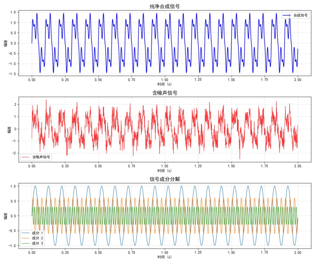
2. Fourier Analysis
def analyze_frequency(signal, sample_rate=1000):
    """
    Perform Fourier analysis on the signal
    """
    n = len(signal)
    # Calculate FFT
    fft_result = np.fft.fft(signal)
    # Calculate frequency axis
    frequencies = np.fft.fftfreq(n, 1/sample_rate)
    # Take positive frequency part
    positive_freq_idx = frequencies > 0
    frequencies = frequencies[positive_freq_idx]
    fft_result = fft_result[positive_freq_idx]
    return frequencies, np.abs(fft_result)
# Analyze clean and noisy signals in the frequency domain
freq_clean, fft_clean = analyze_frequency(clean_signal)
freq_noisy, fft_noisy = analyze_frequency(noisy_signal)
plt.figure(figsize=(12, 8))
plt.subplot(2, 1, 1)
plt.plot(freq_clean, fft_clean)
plt.title('Frequency Spectrum of Clean Signal')
plt.xlabel('Frequency (Hz)')
plt.ylabel('Amplitude')
plt.grid(True)
plt.xlim(0, 100)
plt.subplot(2, 1, 2)
plt.plot(freq_noisy, fft_noisy)
plt.title('Frequency Spectrum of Noisy Signal')
plt.xlabel('Frequency (Hz)')
plt.ylabel('Amplitude')
plt.grid(True)
plt.xlim(0, 100)
plt.tight_layout()
plt.show()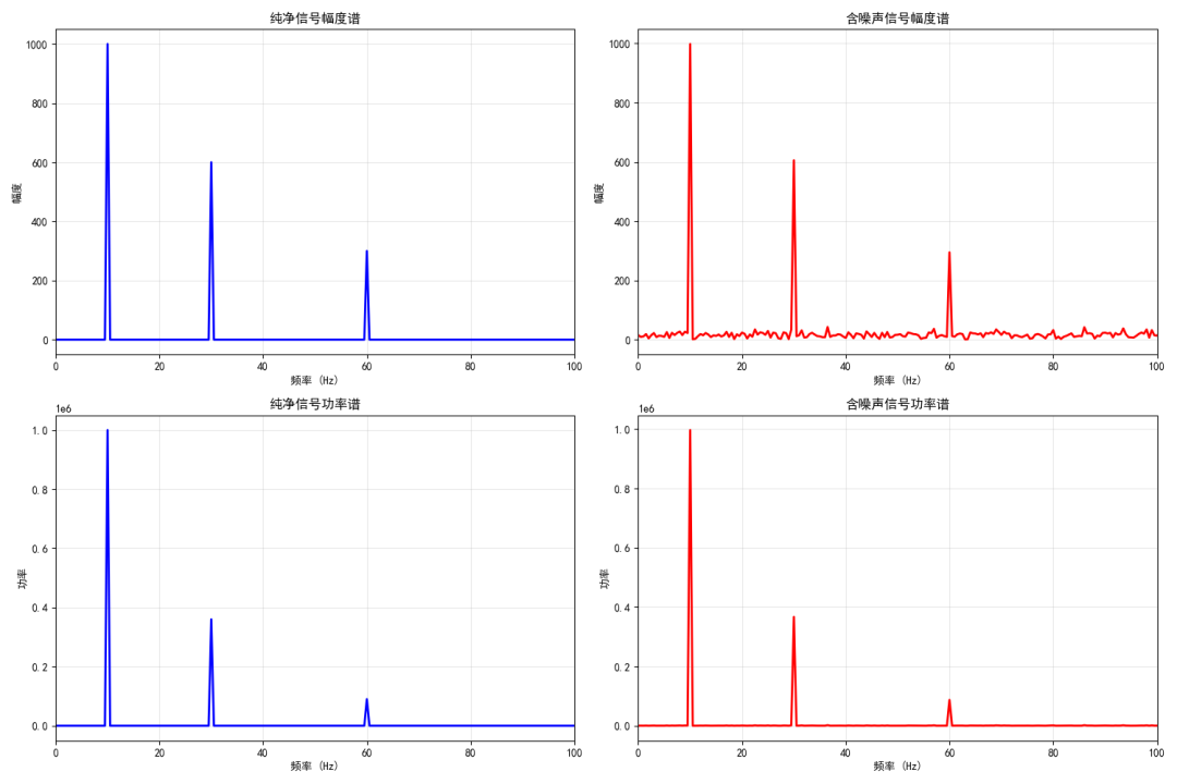
3. Filter Design and Application
def design_filter(lowcut=15, highcut=25, sample_rate=1000, order=5):
    """
    Design a bandpass filter
    """
    nyquist = sample_rate / 2
    low = lowcut / nyquist
    high = highcut / nyquist
    b, a = signal.butter(order, [low, high], btype='band')
    return b, a
def apply_filter(signal, b, a):
    """
    Apply the filter
    """
    return signal.filtfilt(b, a, signal)
# Design filter to extract signals around 20Hz
b, a = design_filter(lowcut=15, highcut=25)
# Apply filter
filtered_signal = apply_filter(noisy_signal, b, a)
plt.figure(figsize=(12, 10))
plt.subplot(3, 1, 1)
plt.plot(t, noisy_signal)
plt.title('Original Noisy Signal')
plt.xlabel('Time (s)')
plt.ylabel('Amplitude')
plt.grid(True)
plt.subplot(3, 1, 2)
plt.plot(t, filtered_signal)
plt.title('Filtered Signal (15-25 Hz Bandpass)')
plt.xlabel('Time (s)')
plt.ylabel('Amplitude')
plt.grid(True)
plt.subplot(3, 1, 3)
# Plot ideal 20Hz signal
ideal_20hz = 0.5 * np.sin(2 * np.pi * 20 * t)
plt.plot(t, ideal_20hz)
plt.title('Ideal 20Hz Signal (for comparison)')
plt.xlabel('Time (s)')
plt.ylabel('Amplitude')
plt.grid(True)
plt.tight_layout()
plt.show()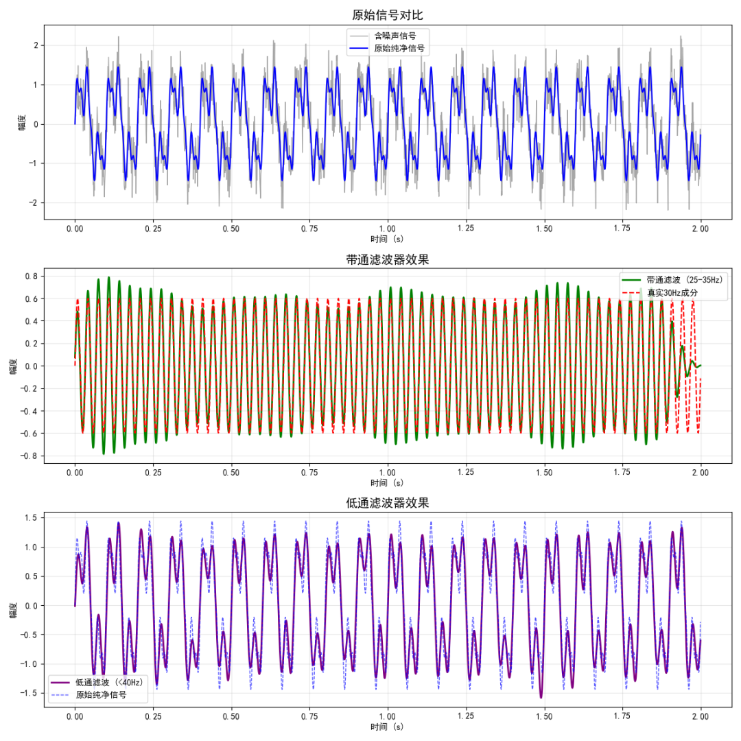
4. Time-Frequency Analysis: Short-Time Fourier Transform
import numpy as np
import matplotlib.pyplot as plt
from scipy import signal
import matplotlib
# Set Chinese font
matplotlib.rcParams['font.sans-serif'] = ['SimHei']
matplotlib.rcParams['axes.unicode_minus'] = False
def plot_spectrogram_analysis(signal_data, sample_rate=1000):
    """
    Plot the time-frequency analysis of the signal
    """
    fig, axes = plt.subplots(1, 2, figsize=(15, 6))
    # Calculate spectrogram
    f, t_spec, Sxx = signal.spectrogram(signal_data, sample_rate,                                       nperseg=256, noverlap=128)
    # Plot spectrogram
    im = axes[0].pcolormesh(t_spec, f, 10 * np.log10(Sxx + 1e-10),                           shading='gouraud', cmap='viridis')
    plt.colorbar(im, ax=axes[0], label='Power Spectral Density (dB)')
    axes[0].set_title('Spectrogram', fontsize=14, fontweight='bold')
    axes[0].set_xlabel('Time (s)')
    axes[0].set_ylabel('Frequency (Hz)')
    axes[0].set_ylim(0, 100)
    # Plot 3D time-frequency graph
    from mpl_toolkits.mplot3d import Axes3D
    # Create grid
    T, F = np.meshgrid(t_spec, f)
    ax = fig.add_subplot(122, projection='3d')
    surf = ax.plot_surface(T, F, 10 * np.log10(Sxx + 1e-10),                          cmap='viridis', alpha=0.8)
    ax.set_title('3D Time-Frequency Analysis', fontsize=14, fontweight='bold')
    ax.set_xlabel('Time (s)')
    ax.set_ylabel('Frequency (Hz)')
    ax.set_zlabel('Amplitude (dB)')
    ax.view_init(30, 45)
    plt.tight_layout()    plt.show()
# Generate test signal
def generate_test_signal():
    """Generate a test signal for time-frequency analysis"""
    duration = 2.0
    sample_rate = 1000
    t = np.linspace(0, duration, int(sample_rate * duration), endpoint=False)
    # Create frequency-varying signal
    # Linear chirp signal
    chirp_signal = signal.chirp(t, f0=10, f1=80, t1=duration, method='linear')
    # Add some transient components
    transient_signal = np.zeros_like(t)
    transient_times = [0.5, 1.0, 1.5]  # seconds
    for trans_time in transient_times:
        idx = int(trans_time * sample_rate)
        transient_signal[idx:idx+100] = 1.0
    # Composite signal
    composite_signal = chirp_signal + 0.3 * transient_signal + 0.1 * np.random.normal(size=t.shape)
    return t, composite_signal
# Run time-frequency analysis
print("Performing time-frequency analysis...")
t, test_signal = generate_test_signal()
plot_spectrogram_analysis(test_signal)
print("Time-frequency analysis completed!")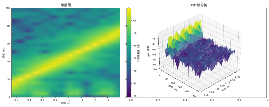
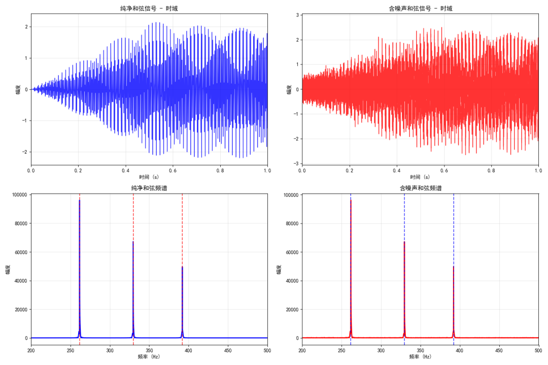
5. Practical Application: Audio Signal Processing Simulation
def simulate_audio_processing():
    """
    Simulate audio signal processing
    """
    # Create a longer signal to simulate audio
    duration = 5.0
    sample_rate = 44100
    t_audio = np.linspace(0, duration, int(sample_rate * duration))
    # Create chord signal (C major chord: C4, E4, G4)
    frequencies = [261.63, 329.63, 392.00]  # C4, E4, G4
    amplitudes = [1.0, 0.7, 0.5]
    chord_signal = np.zeros_like(t_audio)
    for freq, amp in zip(frequencies, amplitudes):
        chord_signal += amp * np.sin(2 * np.pi * freq * t_audio)
    # Add envelope
    envelope = np.ones_like(t_audio)
    attack = int(0.5 * sample_rate)
    release = int(0.5 * sample_rate)
    sustain = len(t_audio) - attack - release
    envelope[:attack] = np.linspace(0, 1, attack)
    envelope[attack:attack+sustain] = 1
    envelope[attack+sustain:] = np.linspace(1, 0, release)
    chord_signal *= envelope
    noisy_chord = chord_signal + 0.2 * np.random.normal(size=chord_signal.shape)
    return t_audio, chord_signal, noisy_chord, frequencies
# Generate simulated audio signal
t_audio, chord_clean, chord_noisy, note_freqs = simulate_audio_processing()
# Analyze audio signal
fig, axes = plt.subplots(2, 2, figsize=(15, 10))
# Time domain signal
axes[0, 0].plot(t_audio, chord_clean, 'b-', linewidth=1, alpha=0.8)
axes[0, 0].set_title('Clean Chord Signal - Time Domain', fontsize=12, fontweight='bold')
axes[0, 0].set_xlabel('Time (s)')
axes[0, 0].set_ylabel('Amplitude')
axes[0, 0].grid(True, alpha=0.3)
axes[0, 0].set_xlim(0, 1)  # Show only the first second
axes[0, 1].plot(t_audio, chord_noisy, 'r-', linewidth=1, alpha=0.8)
axes[0, 1].set_title('Noisy Chord Signal - Time Domain', fontsize=12, fontweight='bold')
axes[0, 1].set_xlabel('Time (s)')
axes[0, 1].set_ylabel('Amplitude')
axes[0, 1].grid(True, alpha=0.3)
axes[0, 1].set_xlim(0, 1)
# Frequency domain analysis
freq_audio, mag_audio, _ = frequency_analysis(chord_clean, 44100)
freq_noisy_audio, mag_noisy_audio, _ = frequency_analysis(chord_noisy, 44100)
axes[1, 0].plot(freq_audio, mag_audio, 'b-', linewidth=2)
# Mark note frequencies
for freq in note_freqs:
    axes[1, 0].axvline(x=freq, color='red', linestyle='--', alpha=0.7,                       label=f'{freq:.1f}Hz')
axes[1, 0].set_title('Frequency Spectrum of Clean Chord', fontsize=12, fontweight='bold')
axes[1, 0].set_xlabel('Frequency (Hz)')
axes[1, 0].set_ylabel('Amplitude')
axes[1, 0].grid(True, alpha=0.3)
axes[1, 0].set_xlim(200, 500)
axes[1, 1].plot(freq_noisy_audio, mag_noisy_audio, 'r-', linewidth=2)
for freq in note_freqs:
    axes[1, 1].axvline(x=freq, color='blue', linestyle='--', alpha=0.7)
axes[1, 1].set_title('Frequency Spectrum of Noisy Chord', fontsize=12, fontweight='bold')
axes[1, 1].set_xlabel('Frequency (Hz)')
axes[1, 1].set_ylabel('Amplitude')
axes[1, 1].grid(True, alpha=0.3)
axes[1, 1].set_xlim(200, 500)
plt.tight_layout()
plt.show()