Spatial Data Prediction Based on Python: Random Forest Model Method (Part 1)

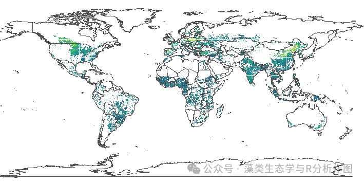
When we collect global sample data, we often want to extrapolate the entire global pattern. For example, the core analysis in the NC article titled “Soil organic carbon thresholds control fertilizer effects on carbon accrual in croplands worldwide”:From the measured data in Figure a, a global 10km resolution raster file is predicted based on the Random Forest model: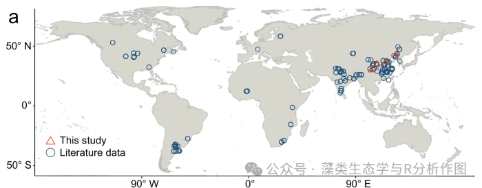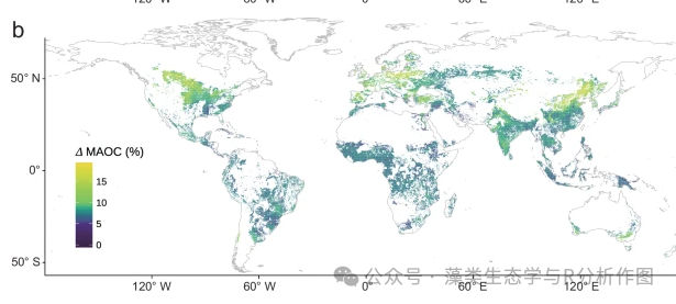The basic principle is to use existing observation point data + climate/environmental factors, divided into 25% / 75% for training and validation sets, to train a relationship model, and then apply this model to areas “without observations” to calculate the predicted values using the climate/environmental factors.Currently, there are many common modeling methods:

• Random Forest

• LightGBM

• XGBoost

• CatBoost

• Support Vector Machine

…..This article will first introduce the most commonly used model: Random Forest. The code and steps for the other models will be published in upcoming posts, so stay tuned.Preparing climate/environmental factor data:First, we need to align and extract the raster files of climate/environmental factors. For specific steps, please refer to previous posts on this public account:

Resampling

George, Public Account: Algal Ecology and R Analysis Resampling of Geographic Raster Images (Aligning Resolution)

Then, we need to convert the raster files into xlsx files. For specific steps, please refer to previous posts on this public account:

Format Conversion

George, Public Account: Algal Ecology and R Analysis Predicting Raster Data under Future Climate Scenarios Based on R + Random Forest Model

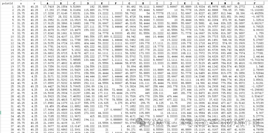
Then we obtain today’s global scale climate/environmental factors A-P: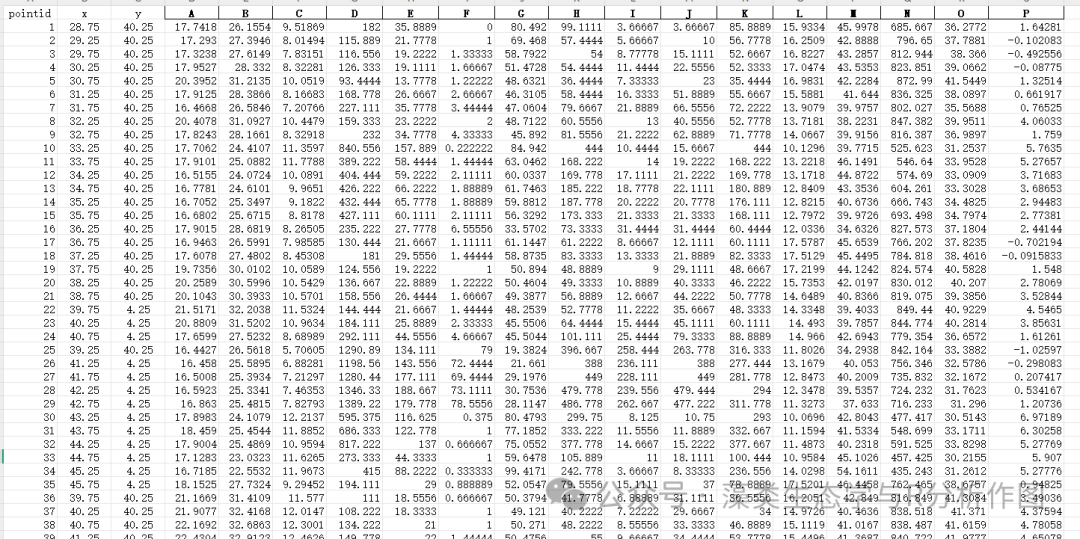Next, we prepare the actual sampling point data and the paired environmental factor data, dividing them into two groups:

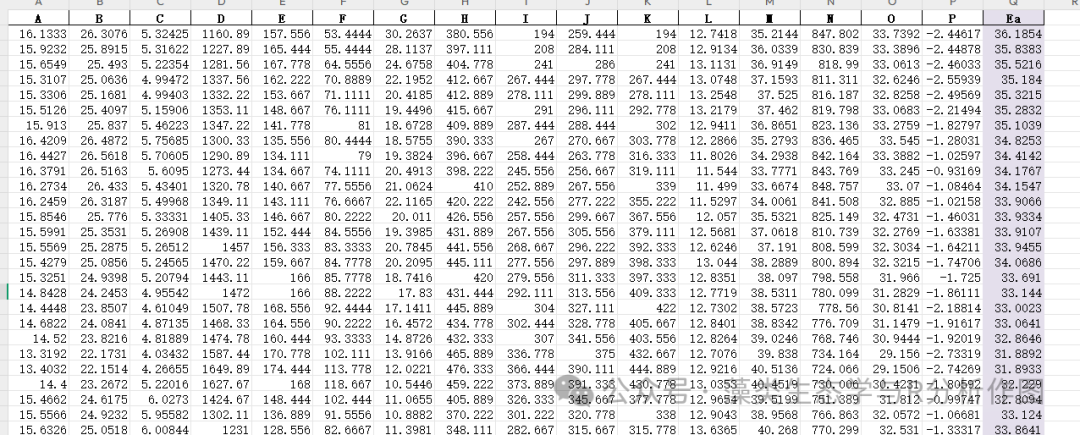
Training Data (training_set_with_data_augmentation.xlsx): 75%

Validation Data (test_set.xlsx): 25%

A-P is our climate environmental factor, and Ea is our predicted data today. The training and validation files are in the same format:

Then, we start configuring the environment:

The following analysis requires Python 3+. First, change the interpreter settings in PyCharm:

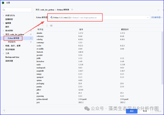
Then, remember this location, click on your computer’swin+R, inputCMD, and in the interface input:

"C:\Python27\.venv\Scripts\python.exe" -m ensurepip"C:\Python27\.venv\Scripts\python.exe" -m pip install --upgrade pip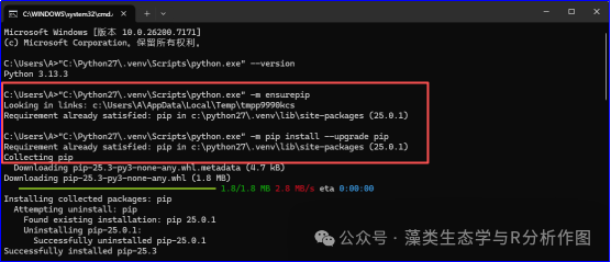

Continue installing:

"C:\Python27\.venv\Scripts\python.exe" -m pip install scikit-learn pandas matplotlib numpy optuna openpyxl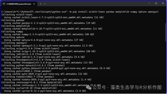

Then return to PyCharm, and in the terminal below, input the code. Please be patient and ensure that the magic support is set up:

pip install pandas numpy matplotlib scikit-learn optuna lightgbm xgboost catboost openpyxl

When the following content pops up, it indicates that all installations were successful: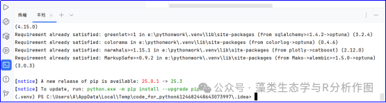Start executing the code:First, start training the model:

# Import evaluation metrics from sklearn: R², MSE, EVS, MAE
from sklearn.metrics import r2_score as R2
from sklearn.metrics import mean_squared_error as MSE
from sklearn.metrics import explained_variance_score as EVS
from sklearn.metrics import mean_absolute_error as MAE
# Import model from sklearn: RandomForestRegressor; pandas: read Excel; matplotlib.pyplot: plot; numpy: perform array calculations; KFold: cross-validation; optuna: automatic parameter tuning tool
from sklearn.ensemble import RandomForestRegressor
import pandas as pd
from matplotlib import pyplot as plt
import numpy as np
from sklearn.model_selection import KFold
import optuna
#warnings: suppress annoying future warnings → turn off
import warnings
# First line: hide FutureWarning
warnings.filterwarnings("ignore", category=FutureWarning)
# Second line: set the font and size for plotting (Times New Roman, size 20)
plt.rc('font', family='Times New Roman', size=20)
# We define two files, one for the training set and one for the validation set. They contain explanatory factors ABCD... and the predicted factor Ea
train_path = r'E:\land\training_set_with_data_augmentation.xlsx'
test_path  = r'E:\land\test_set.xlsx'
train_data = pd.read_excel(train_path)
test_data = pd.read_excel(test_path)
# X_columns: you tell the model that these 16 columns are features (independent variables)
# y_column: this column is the target (dependent variable), which you want to predict
X_columns = ['A', 'B', 'C', 'D', 'E', 'F', 'G', 'H', 'I', 'J', 'K', 'L', 'M', 'N', 'O', 'P']
y_column = 'Ea'
X_train = train_data[X_columns].values
y_train = train_data[y_column].values
X_test = test_data[X_columns].values
y_test = test_data[y_column].values
# Define 5-fold cross-validation: i.e., divide the training set into 5 parts, using 4 parts for training and 1 part for validation, looping 5 times, taking the average R² as the performance of "this set of parameters". shuffle=True: shuffle the data before splitting. random_state=2024: set the random seed to ensure consistent results across different computers.
kf = KFold(n_splits=5, random_state=2024, shuffle=True)
# Optuna automatic parameter tuning: i.e., repeatedly perform 5-fold cross-validation to obtain R², Optuna will remember which set of parameters has the highest R².
def objective_function(trial):    # 1) Optuna: this step sets the initial parameters for the Random Forest model, no need to modify
    max_depth = trial.suggest_int('max_depth', 1, 20)
    n_estimators = trial.suggest_int('n_estimators', 10, 1000)
    min_samples_split = trial.suggest_int('min_samples_split', 2, 10)
    random_state = trial.suggest_int('random_state', 0, 3000)
    # 2) Build a Random Forest model with this set of parameters
    rf = RandomForestRegressor(max_depth=max_depth,                               n_estimators=n_estimators,                               min_samples_split=min_samples_split,                               random_state=random_state)
    # 3) Perform 5-fold cross-validation
    scores = []
    for train_idx, val_idx in kf.split(X_train):        X_train_fold, X_val_fold = X_train[train_idx], X_train[val_idx]        y_train_fold, y_val_fold = y_train[train_idx], y_train[val_idx]        rf.fit(X_train_fold, y_train_fold)             y_pred_fold = rf.predict(X_val_fold)           fold_score = R2(y_val_fold, y_pred_fold)          scores.append(fold_score)    # 4) Return the average R² of 5 folds, the larger the R², the better
    return np.mean(scores)
###### Officially start parameter tuning: this step requires patience ########### To avoid repeatedly running this parameter tuning step, we can comment out the code below after successfully tuning it once, and directly use the best parameters
study = optuna.create_study(direction='maximize')   # Objective: maximize R²
n_trials = 200  # Hyperparameter attempts for 200 rounds (if this step takes too long, you can modify it to 100 or another number to see the effect, to save time, we set the sample data to 20)
study.optimize(objective_function, n_trials=n_trials)
best_params = study.best_trial.params    # This step is the set of "parameters with the highest average R²"
print('Best hyperparameters:', best_params)
# This step will automatically display each step's parameters in the output area:
# We can find that the R² is around 0.53, and the current best parameters are: 'max_depth': 16; 'n_estimators': 845; 'min_samples_split': 2; 'random_state': 2038}
# Directly adopt the best parameters generated earlier and continue with the following operations
# best_params = study.best_trial.params
# Or, if we do not want to repeatedly execute the optimal tuning step above, we can comment out
# the tuning code above and directly input the best parameters we just obtained:
best_params = {    'max_depth': 16,    'n_estimators': 845,    'min_samples_split': 2,    'random_state': 2038}
# Start officially running the Random Forest model:
rf = RandomForestRegressor(max_depth=best_params['max_depth'],                           n_estimators=best_params['n_estimators'],                           min_samples_split=best_params['min_samples_split'],                           random_state=best_params['random_state'])
rf.fit(X_train, y_train)         # Fit again using the entire training set
y_pred = rf.predict(X_test)      # Predict on the test set
# Calculate various evaluation metrics
mae = MAE(y_test, y_pred)
mse = MSE(y_test, y_pred)
rmse = np.sqrt(mse)
ev = EVS(y_test, y_pred)
r2 = R2(y_test, y_pred)
print('\nRandomForest Evaluation Metrics:')
print('MAE:', mae)
print('MSE:', mse)
print('RMSE:', rmse)
print('EVS:', evs)
print('R2:', r2)

# MAE: The average absolute difference between predicted and true values → the smaller, the better, the unit is consistent with the unit of Ea# MSE: The average of the squared prediction errors → the smaller, the better# RMSE: The square root of MSE → the smaller, the better# EVS: Explained variance, the closer to 1, the better# R2: Coefficient of determination, the closer to 1, the better, 0 is very poor, negative = very poorOutput the model:

# Plot True vs Prediction scatter plot
# Set the figure's length, width, and resolution
plt.figure(figsize=(10, 8), dpi=100) # Scatter plot: true values on the x-axis, predicted values on the y-axis
plt.scatter(y_test, y_pred, color='black') # Calculate the coordinate axis range (the common min/max values of true and predicted values)
min_val = min(y_test.min(), y_pred.min())
max_val = max(y_test.max(), y_pred.max()) # Draw the diagonal dashed line y = x (ideal line for perfect prediction)
plt.plot([min_val, max_val], [min_val, max_val],         linestyle='dashed', color='royalblue') # Make x and y coordinate ranges consistent
plt.xlim(min_val, max_val)
plt.ylim(min_val, max_val) plt.xlabel('True')
plt.ylabel('Prediction')
plt.title('True vs Predicted (Test set)')
plt.gca().set_aspect('equal', 'box') # Save as PDF to E:\land
pdf_path = r"E:\land\Ea_true_vs_pred.pdf" 
plt.savefig(pdf_path, format="pdf", bbox_inches="tight")
plt.show()   # This step will pop up a scatter plot window, Python will keep running, manually close the window to indicate completion
# Output model file:
import pickle
with open(r'model_save/RandomForest.model', 'wb') as file:    pickle.dump(rf, file)

At this point, we have obtained our trained model: RandomForest.model fileNext, we will use the global scale climate/environmental factors + RandomForest.model to predict the global scale Ea data:Create a new .py file window:

import os
import pickle
import pandas as pd
import numpy as np 
folder = r"E:\land"            # Folder where the model and data are located
model_filename = "RandomForest.model"   # Your saved model name
data_filename = "data.xlsx"            # New data to be predicted 
model_path = os.path.join(folder, model_filename)
data_path = os.path.join(folder, data_filename) # Read the model
with open(model_path, "rb") as f:    model = pickle.load(f) 
df = pd.read_excel(data_path)  # Default reads the first sheet 
# Prepare feature matrix (must be consistent with features during training)
X_columns = ['A', 'B', 'C', 'D', 'E', 'F', 'G', 'H',             'I', 'J', 'K', 'L', 'M', 'N', 'O', 'P'] 
X_new = df[X_columns].values # Extrapolate prediction
y_pred = model.predict(X_new)
df["Ea_pred"] = y_pred   # Add a column for predicted values
print(df.head()) 
out_xlsx = os.path.join(folder, "data_with_prediction.xlsx")
df.to_excel(out_xlsx, index=False)
print("  Excel:", out_xlsx)

Output the predicted global scale Ea data: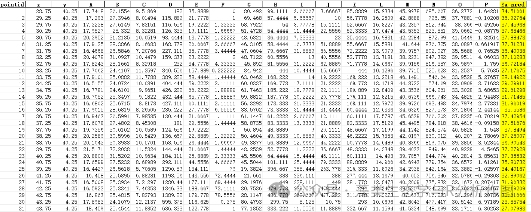After obtaining the data, we can convert the predicted Ea data into raster files based on the code from previous posts:

Convert Raster

George, Public Account: Algal Ecology and R Analysis Predicting Raster Data under Future Climate Scenarios Based on R + Random Forest Model

Over~It is the reason, the result, and the process.