1. Generating Input Waveforms for FIR IP in Matlab

2. Generating Filter Coefficients for FIR IP in Matlab
In FPGA-based digital signal processing, data transfer and simulation verification between Matlab, Vivado, and Modelsim are required. The typical approach is for Matlab to generate input signals for the Verilog module as simulation stimuli, followed by testing the functionality of the algorithm module using Vivado and Modelsim (or other Verilog development platforms), and finally importing the output signals from Verilog back into Matlab for comparison and verification.
The overall engineering design approach and specific steps are as follows:
① In Matlab, a 15MHz single-tone signal and a 5MHz single-tone signal are combined to create a mixed signal as the input signal for the FPGA’s FIR. The sampling rate is set to 100MHz, and an 8MHz low-pass FIR filter is designed, exporting the FIR filter coefficients and the binary values of the mixed signal;
② The FIR IP data filtering process in the FPGA uses the 8MHz low-pass filter to obtain the filtered simulation data of the 5MHz signal;
③ The simulation data from Vivado and Modelsim is imported into Matlab for FFT processing to analyze and compare whether the data meets design requirements.
1. Generating Input Waveforms for FIR IP in Matlab
By constructing a waveform generation function, the simulated signal is quantized to 12 bits and stored in binary format corresponding to the waveform. The quantized signal undergoes FFT Fourier transform processing to obtain the amplitude spectrum for analysis and comparison. The waveform generation code in Matlab is as follows:
function [u_yt,yt] = wave_gen(fid,ADC_bit,L,st)

y=st/max(abs(st));                 % Normalization
yt=round(y*(2^(ADC_bit-1)-1));     % 12-bit quantization  round() indicates rounding
YT_FFT=fft(yt,L);   % Fourier transform
P_YT=abs(YT_FFT)/L; % Amplitude spectrum
u_yt=max(P_YT);     % Get the amplitude value of the signal received by beam 1

for p=1:L
    B_s=dec2bin(yt(p)+(yt(p)<0)*2^ADC_bit,ADC_bit);
    for q=1:ADC_bit  % 12 bits, sequentially checking the values of these 12 bits
        if B_s(q)=='1'
            data=1;
        else
            data=0;
        end
        fprintf(fid,'%d',data);
    end
    fprintf(fid,'\r\n');
end
fclose(fid);
end
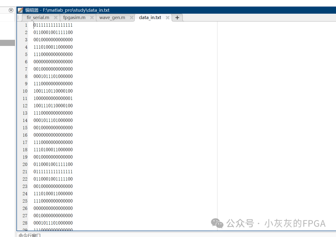
The Matlab code implements the output of the mixed signal, which serves as the input stimulus for FPGA testing and simulation. The 5MHz single-tone signal and the 5MHz single-tone signal are combined to create a mixed signal as the input signal for the FPGA’s FIR, with a sampling rate of 100MHz, and the data is saved to the data_in.txt file.
The specific Matlab code is as follows:
close all;
clear all;
clc;
%%%%%%%%%%%%%%%%%%%%%%%%%%%%%%%%%%%%%%%
%           Parameter Definition
%%%%%%%%%%%%%%%%%%%%%%%%%%%%%%%%%%%%%%%
ADC_bit=16;      % Sampling bit depth
N=1024;          % Number of samples

f1=5e6;          % Signal frequency 1 5M
f2=15e6;         % Signal frequency 2 15M
fs=100e6;         % Sampling frequency
t=0:1/fs:(N-1)/fs;
st=cos(2*pi*f1*t)+cos(2*pi*f2*t);

% Amplitude spectrum
P_st=fftshift(fft(st));
P_st=abs(P_st)/N;
f=(0:N-1)*fs/N-fs/2;

figure(1)
subplot(211);
plot(t,st);hold on;
subplot(212);
plot(f/1e6,P_st);grid on;        % Frequency points appear at f and fs-f
title('FFT Transformation');
xlabel('Frequency/MHz');ylabel('Amplitude');
%%%%%%%%%%%%%%%%%%%%%%%%%%%%%%%%%%%%%%%
%             Export Waveform Data
%%%%%%%%%%%%%%%%%%%%%%%%%%%%%%%%%%%%%%%
fid=fopen('data_in.txt','w');
[u_x1_real,x1_real]= wave_gen(fid,ADC_bit,N,real(st) );
fprintf('x1_real signal amplitude value is %g\n',u_x1_real);

figure(2)
% plot(t,st);hold on;
plot(t,x1_real);hold on;
The generated text data format is as follows:
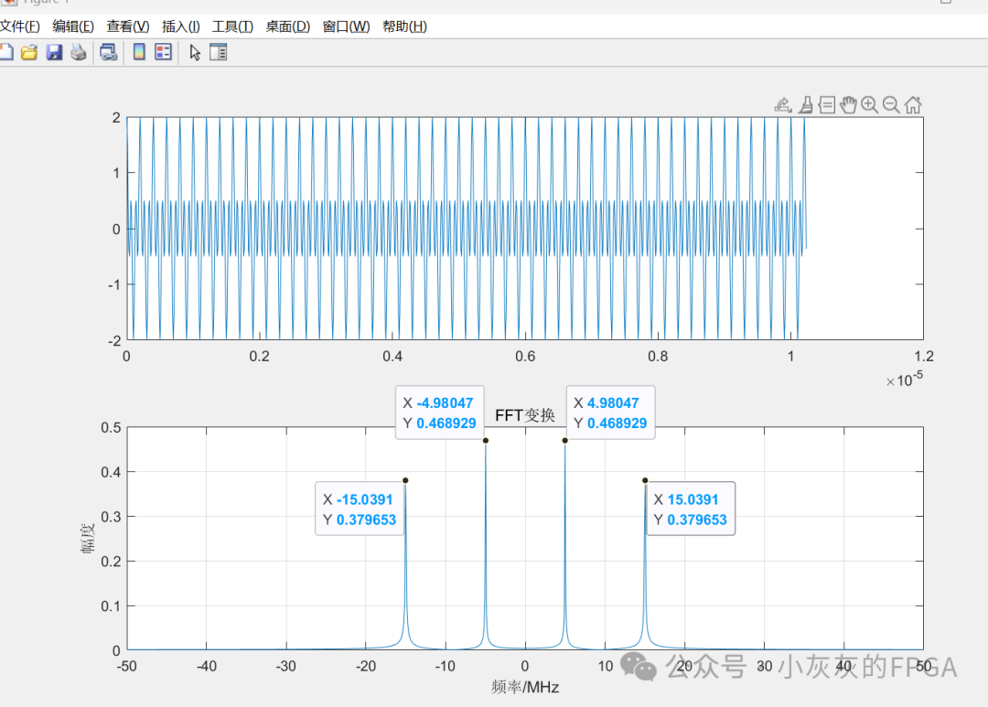
The time-domain and frequency-domain data graphs of the generated mixed signal are as follows:
 2. Generating Filter Coefficients for FIR IP in Matlab
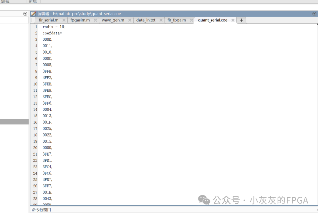
In Matlab, the fir1 function is used to design an 8MHz low-pass FIR filter, quantize the filter coefficients, and export the FIR filter coefficients, saving them to a .coe file.
The specific Matlab code is as follows:
close all;
clear all;
clc;
N=160;      % Filter length
fs=100e6;   % Sampling frequency
fc=8e6;    % Cut-off frequency of the low-pass filter
B=14;      % Quantization bit depth

% Generate Hamming window
w_hamm=hamming(N);
% Design FIR filter using fir1 function
b_hamm=fir1(N-1,fc*2/fs,'low',w_hamm);
% Quantize filter coefficients
Q_hamm=round(b_hamm/max(abs(b_hamm))*(2^(B-1)-1));
% Convert to hexadecimal two's complement
Q_h=dec2hex(Q_hamm+2^B*(Q_hamm<0));

% Write the generated filter coefficient data to the COE file required by FPGA
fid=fopen('F:\matlab_pro\study\quant_serial.coe','w');
fprintf(fid,'radix = 16;\r\n');
fprintf(fid,'coefdata=\r\n');
for i = 1:size(Q_h,1)
    if i == size(Q_h,1)
        fprintf(fid,'%s;\n',Q_h(i,:));
    else
        fprintf(fid,'%s,\n',Q_h(i,:));
    end
end
%fprintf(fid,'%x\r\n',Q_h);
fclose(fid);
The FIR filter coefficient file is as follows: