💥💥💞💞 Welcome to this blog ❤️❤️💥💥
🏆 Blogger’s Advantage: 🌞🌞🌞 The blog content aims to be logically clear and coherent for the convenience of readers.
⛳️ Motto: A journey of a hundred miles begins with a single step.
📋📋📋 The content of this article is as follows: 🎁🎁🎁
⛳️ A gift to readers
👨💻 Conducting research involves a profound system of thought, requiring researchers to be logical, diligent, and serious. However, effort alone is not enough; often leveraging resources is more important than sheer effort. Additionally, one should have innovative and inspirational points of view. It is recommended that readers browse through the content in order to avoid suddenly falling into a dark maze without finding their way back. This may not reveal all the answers to your questions, but if it can clarify the clouds of doubt rising in your mind, it may create a beautiful sunset of insights. If it brings you a storm in your spiritual world, then take the opportunity to brush off the dust that has settled on your ‘lying flat’ mindset.
Perhaps, after the rain, the sky will be clearer… 🔎🔎🔎
1 Interior Point Method
The interior point method is a type of constrained optimization algorithm. The basic idea of constrained optimization algorithms is to transform the constrained optimization problem into an unconstrained problem by introducing a utility function, and then continuously update the utility function through the optimization iteration process to ensure convergence of the algorithm. The main idea of the interior point method (a type of penalty function method) is to build a high “wall” at the boundary of the feasible region. When the iteration point approaches the boundary, the objective function increases significantly as a form of punishment, preventing the iteration point from crossing the boundary, thus keeping the optimal solution within the feasible region. Detailed explanation: Interior Point Method
2 Overview of Optimal Power Flow
2.1 Overview
Comparing optimal power flow with basic power flow, power flow calculations can be summarized as determining the corresponding state variables x (such as node voltage magnitudes and angles) based on certain disturbance variables p (load conditions) and given control variables u (such as generator active power output, reactive power output, or node voltage magnitudes). The power flow solution obtained from a single power flow calculation determines a specific operating state of the power system. This type of power flow calculation can also be referred to as basic power flow (or conventional power flow) calculation, where the results primarily satisfy the power flow equations or equality constraints among variables:
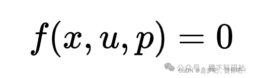

The operating state determined by a single power flow calculation may not be feasible due to certain state variables or other variables as functions of u and x exceeding their permissible operating limits (i.e., not satisfying inequality constraints). The common engineering approach is to adjust the given values of certain control variables and re-conduct the aforementioned basic power flow calculation, repeating this process until all constraints are satisfied. This results in a technically feasible power flow solution.
Since there is a certain gap between the upper and lower limits of the system’s state variables and related function variables, and control variables can also be adjusted within their permissible ranges, theoretically, for a given load condition, there can exist numerous feasible power flow solutions that technically meet the requirements. Each feasible power flow solution corresponds to a specific operating mode of the system, with corresponding overall economic or technical performance indicators (such as total fuel consumption of the system, total network losses, etc.). To optimize system operation, it is necessary to select the best performance indicator from all feasible power flow solutions. This is the problem that optimal power flow aims to solve.
Therefore, the so-called optimal power flow is the power flow distribution found through the optimal selection of control variables when the system’s structural parameters and load conditions are given, which satisfies all specified constraints and optimizes a certain performance indicator or objective function of the system.
2.2 Comparison of Optimal Power Flow and Basic Power Flow
(1) In basic power flow calculations, the control variables u are predetermined; while in optimal power flow, u is a variable to be optimized, thus there must be an objective function serving as the optimization criterion for u in the optimal power flow model.
(2) In addition to satisfying the power flow equations as equality constraints, optimal power flow calculations must also meet a large number of inequality constraints related to operational limits.
(3) Basic power flow calculations solve a system of nonlinear algebraic equations; while optimal power flow calculations, from a mathematical perspective, are a nonlinear programming problem, thus requiring optimization methods for solution.
(4) Basic power flow calculations only perform a computational function, i.e., determining the corresponding x from the given u; while optimal power flow calculations can automatically optimize control variables based on a specific objective function while satisfying corresponding constraints, thus providing a decision-making function for guiding system optimization adjustments.
2.3 Interior Point Method for Optimal Power Flow Calculation
The interior point method is a method for optimization within the feasible region. In 1984, Karmarkar proposed the interior point method, which has polynomial computational complexity and is over 50 times faster than the simplex method when solving large-scale linear programming problems. In 1986, Gill extended the interior point method to the field of nonlinear programming.
(1) Basic Idea
The initial basic idea of the interior point method is to ensure that the optimization iteration process always occurs within the feasible region. Therefore, the initial point should be taken within the feasible region, and “barriers” should be set at the boundary of the feasible region to keep the iteration points as interior points.
(2) Existing Difficulties
However, finding an initial feasible point for actual large-scale systems is relatively difficult.
(3) Improved Method – Center Trajectory Interior Point Method
The center trajectory interior point method improves this by only requiring that the slack variables and Lagrange multipliers satisfy simple conditions of being greater than or less than zero during the optimization process, replacing the original requirement of solving within the feasible region, thus greatly simplifying the computation process.
(4) Detailed Introduction to the Center Trajectory Interior Point Method
-
Basic Mathematical Model of Path Tracking Method
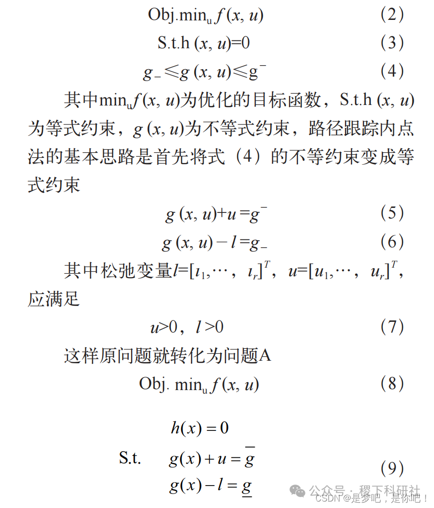

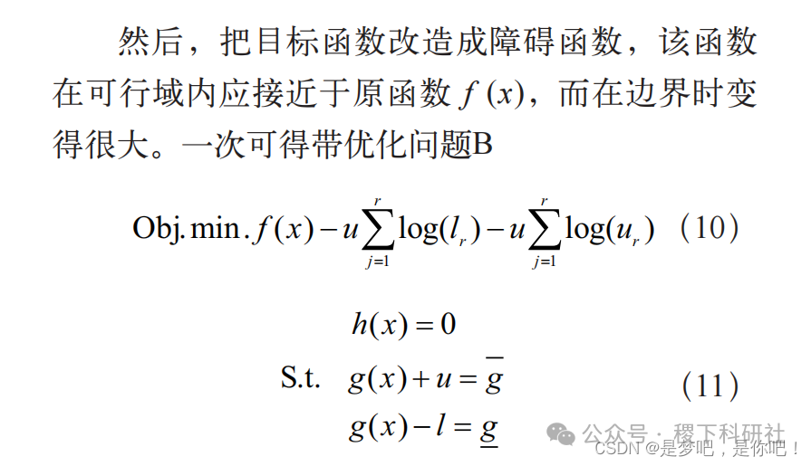

Where the disturbance factor or barrier factor u>0. When l or u approaches the boundary, the above functions will tend to infinity, thus the minimum solution of the above barrier objective function cannot be found on the boundary. This transforms the optimization problem A with inequality constraints into an optimization problem B with only equality constraints, allowing for direct solution using the Lagrange multiplier method.
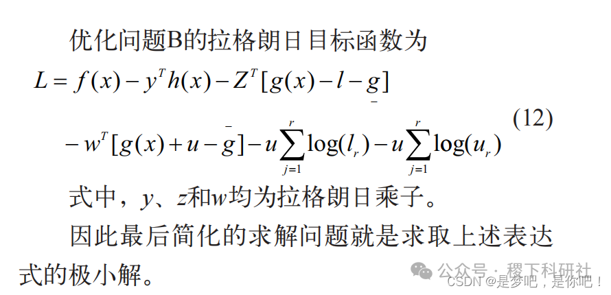

2) Optimal Power Flow Solving Idea of Path Tracking Method
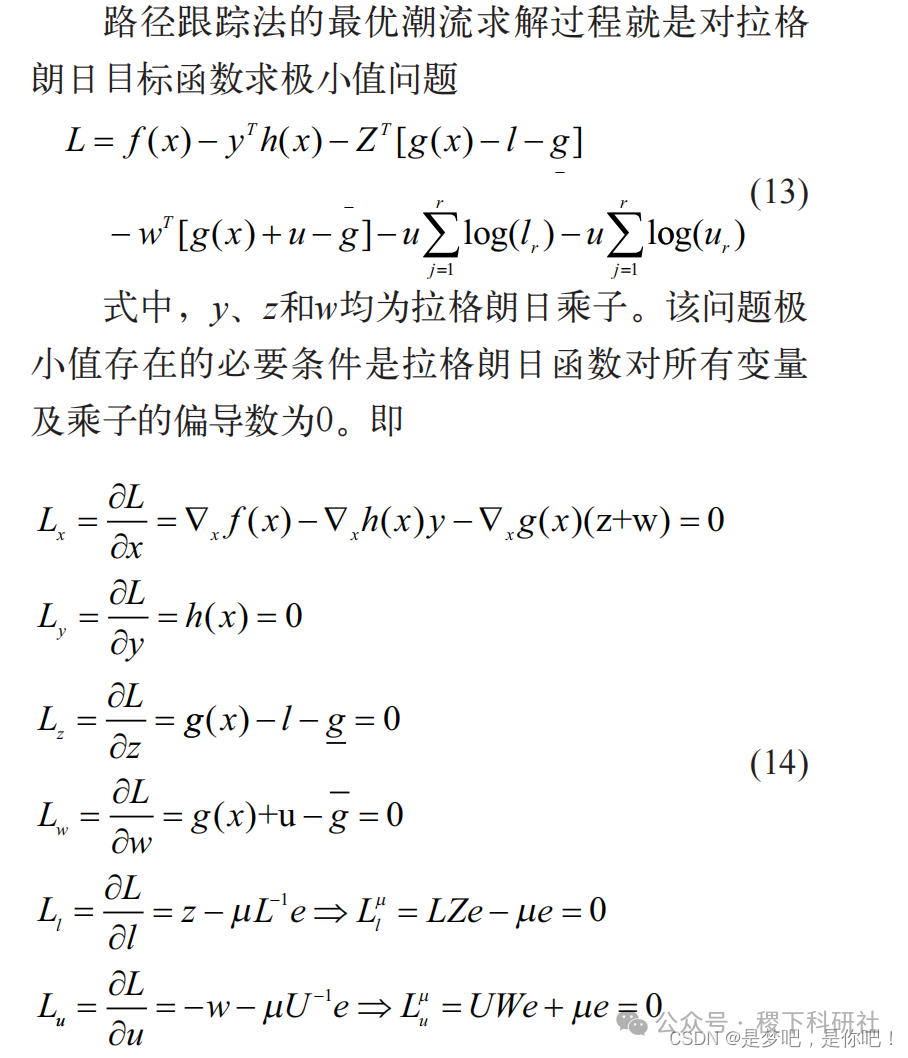
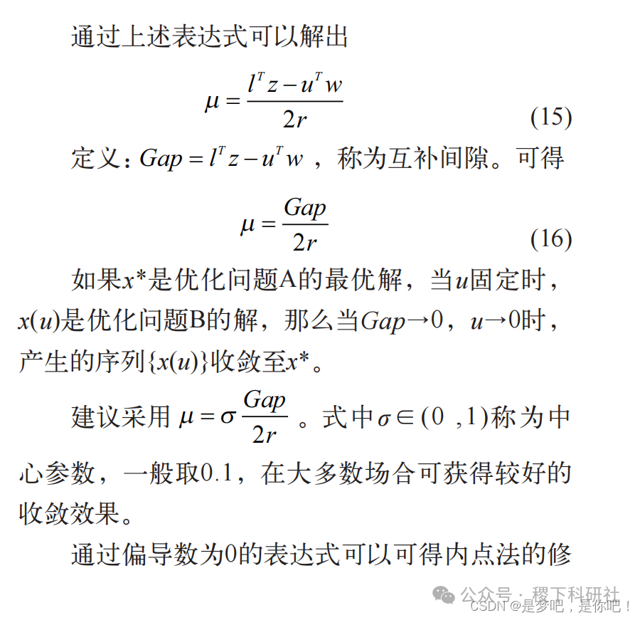
The optimal power flow solving process of the path tracking method is to minimize the Lagrange objective function



3 Example and Program Implementation Process
3.1 Example Description
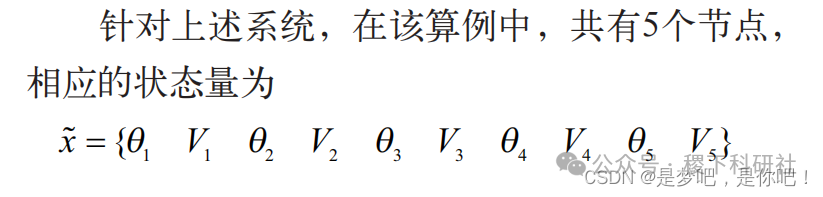
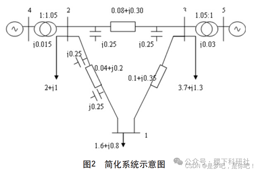
Taking the system fuel cost minimization as the objective function for optimal power flow calculation of the simplified system shown in Figure 2. The line transmission power boundaries, generator active and reactive power upper and lower limits, and fuel cost curve parameters are shown in Tables 1 and 2. All data is presented in per unit form, with a power base value of 100 MV·A, and the upper and lower limits of bus voltage are 1.1 and 0.9, respectively.
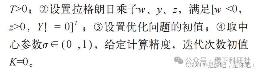
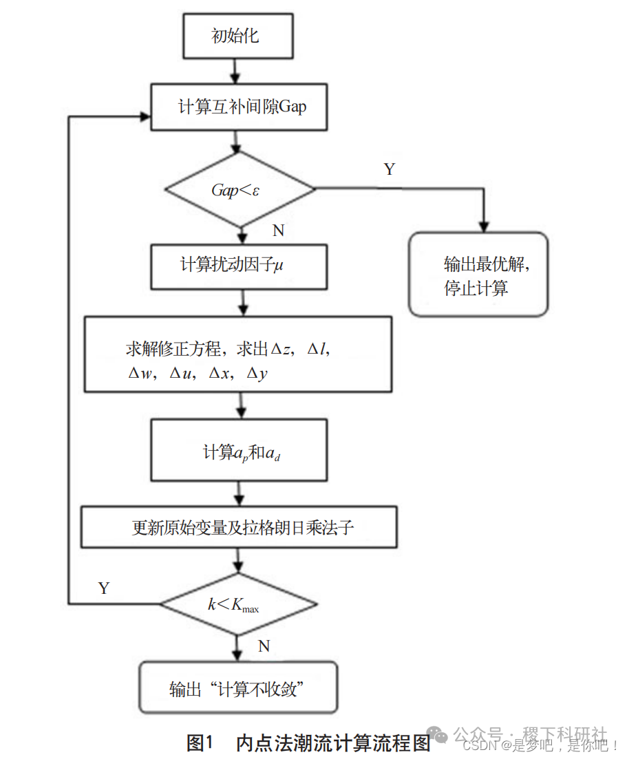
3.2 Specific Implementation Process of the Program


3.3 Case





4 Matlab Implementation
4.1 Main Function
% Optimal Power Flow (OPF) solved by interior point method % Note: This program includes a main file main.m and three function files makeY.m, Coeff.m, and dPQ.m. All four files should be placed in the current MATLAB directory. % Running main.m will print the calculation results to the screen and save them to the file solution.txt. clc; clear; close all; tic; %% Example Data % Node Data Table % 1 2 3 4 5 6 7 8 9 10 11 12 13 14 15 16 17 18 19 % Node Area Type Voltage Phase Angle Active Power Reactive Power Active Power Reactive Power Voltage Reference Upper Limit Lower Limit Conductance Susceptance Control Node Voltage Voltage % No. No. Type Load Load Output Output Base Voltage Upper Limit Lower Limit % 3 represents balance node, 2 represents PV node, 0 represents PQ node N=[ 1 1 0 1.0000 0.00 1.60 0.80 0.00 0.00 230.00 1.032 0.0000 0.0000 0.0000 0.0000 0 1 1.1 0.9 2 1 0 1.0000 0.00 2.00 1.00 0.00 0.00 18.00 1.025 0.0000 0.0000 0.0000 0.0000 0 2 1.1 0.9 3 1 0 1.0000 0.00 3.70 1.30 0.00 0.00 13.80 1.025 0.0000 0.0000 0.0000 0.0000 0 3 1.1 0.9 4 1 2 1.0000 0.00 0.00 0.00 4.50 0.00 230.00 1.026 0.0000 0.0000 0.0000 0.0000 0 4 1.1 0.9 5 1 3 1.0500 0.00 0.00 0.00 4.50 1.45 0.00 0.996 0.0000 0.0000 0.0000 0.0000 0 5 1.1 0.9]; % Branch Data Table %1 2 3 4 5 6 7 8 9 10 11 12 13 14 15 16 17 18 19 20 21 22 % Start End Area Area Type Resistance Reactance Susceptance Branch Rated Power Lower Limit Upper Limit Control Position Transformer Max Phase Shift Min Max Step Size Min Max Branch % Point Point No. No. Route Type Fixed Power Limit Power Limit Power Limit Bus No. Setting Final Transmission Ratio Final Phase Angle Transformation Ratio Transformation Ratio Voltage Voltage No. B=[ 1 2 1 1 1 0 0.040 0.2500 0.50 0. 0. 2. 0 0 1.0 0.0 0.0 0.0 0.0 0.0 0.0 1 1 3 1 1 1 0 0.100 0.3500 0.0 0. 0. 0.65 0 0 1.0 0.0 0.0 0.0 0.0 0.0 0.0 2 2 3 1 1 1 0 0.080 0.3000 0.50 0. 0. 2. 0 0 1.0 0.0 0.0 0.0 0.0 0.0 0.0 3 2 4 1 1 1 1 0.0 0.0150 0.0 0. 0. 6. 0 0 1.050 0.0 0.0 0.0 0.0 0.0 0.0 4 3 5 1 1 1 1 0.0 0.0300 0.0 0. 0. 5. 0 0 1.050 0.0 0.0 0.0 0.0 0.0 0.0 5]; % Generator Data Table % 1 2 3 4 5 6 7 8 9 % Generator Node Active Reactive Active Reactive Quadratic Linear Constant % No. No. Upper Limit Upper Limit Lower Limit Lower Limit Coefficient Coefficient Term Gen=[ 1 4 8.0 3.0 1.0 -3.0 50.4395 200.4335 1200.6485 2 5 8.0 5.0 1.0 -2.1 200.55 500.746 1857.201]; [num_node,~] = size(N); % Number of Nodes [num_branch,~] = size(B); % Number of Branches % Number of Different Types of Nodes num_PQ = 0; num_PV = 0; for k = 1:num_node if (N(k,3) == 0) num_PQ = num_PQ+1; end if (N(k,3) == 2) num_PV = num_PV+1; end end num_gen = num_node-num_PQ; % 2 Number of Generators num_equa = 2*num_node; %10 Number of Equality Constraints m num_inequa = 2*num_gen+num_node+num_branch; %14 Number of Inequality Constraints r num_state = 2*num_gen+2*num_node; % 14 Number of State Variables nPload = N(1:num_PQ,6); Qload = N(1:num_PQ,7); a2 = Gen(:,7); a1 = Gen(:,8); a0 = Gen(:,9); % Consumption Characteristic Polynomial Coefficients A2 = diag(a2); A1 = diag(a1); % Create Diagonal Matrix or Get Diagonal Elements %% Generate Node Admittance Matrix Y = makeY(N, B, num_node, num_branch); %% Parameter Settings PG = N(num_PQ+1:num_node, 8); % Active Power Output QR = N(num_PQ+1:num_node, 9); % Reactive Power Output P_ejec = N(:,8)-N(:,6); Q_ejec = N(:,9)-N(:,7); % Active Output – Active Load, Reactive Xtilde(1:2:num_node*2-1) = (N(:,5))’; Xtilde(2:2:num_node*2) = (N(:,4))’; u = ones(num_inequa,1); l = ones(num_inequa,1); z = ones(1,num_inequa); w = -0.5*ones(1,num_inequa); y = 1E-10*ones(1,num_equa); y(2:2:num_equa) = -1*y(2:2:num_equa); epsi = 1E-6; sigma = 0.1; num_iteration = 0; max_iteration = 50; g_u = [Gen(:,3); Gen(:,4); N(:,18); B(:,12)]; g_l = [Gen(:,5); Gen(:,6); N(:,19); -B(:,12)]; gap_record = zeros(max_iteration,1); for num_iteration = 1:max_iteration gap = l’-z’-u’-w’; gap_record(num_iteration) = gap; if (gap < epsi) disp(‘iterations completed!’); break; end miu = gap*sigma/2/num_inequa; x = [PG; QR; Xtilde’]; % State Variables x X = [z’; l; w’; u; x; y’]; % Variables to be corrected g1 = PG; g2 = QR; % Active Output g1, Reactive Output g2 g3 = (Xtilde(2:2:num_node*2))’; % Node Voltage Magnitudes g3 for k = 1:num_branch % Line Power Flow g4 ii = B(k,1); jj = B(k,2); theta = Xtilde(ii*2-1)-Xtilde(jj*2-1); g4(k,1) = Xtilde(2*ii)*Xtilde(2*jj)*(real(Y(ii,jj))*cos(theta)+imag(Y(ii,jj))*sin(theta))-Xtilde(2*ii)*Xtilde(2*ii)*real(Y(ii,jj)); end g = [g1; g2; g3; g4]; h = zeros(num_node*2,1); for ii = 1:num_node for jj = 1:num_node theta = Xtilde(ii*2-1)-Xtilde(jj*2-1); h(2*ii-1) = h(2*ii-1)-Xtilde(2*ii)*Xtilde(2*jj)*(real(Y(ii,jj))*cos(theta)+imag(Y(ii,jj))*sin(theta)); h(2*ii) = h(2*ii)-Xtilde(2*ii)*Xtilde(2*jj)*(real(Y(ii,jj))*sin(theta)-imag(Y(ii,jj))*cos(theta)); end h(2*ii-1) = h(2*ii-1)+P_ejec(ii); h(2*ii) = h(2*ii)+Q_ejec(ii); end L = diag(l); U = diag(u); Z = diag(z); W = diag(w); % Lagrange Function %% Partial Derivatives of Lagrange Function Ly = h; Lz = g-l-g_l; Lw = g+u-g_u; L_miu_l = L*Z*ones(num_inequa,1)-miu*ones(num_inequa,1); L_miu_u = U*W*ones(num_inequa,1)+miu*ones(num_inequa,1); [A, dh_dx, dg_dx, H_, d2h_dx_y, d2g_dx_c, d2f_dx, temp, L_Z, U_W] = Coeff(num_node, num_PQ, Y, B, X, A2); %% Objective Function df_dx = [2*A2*PG+a1; zeros(2,1); zeros(length(Xtilde),1)]; %% Lagrange Function Lx = df_dx-dh_dx*y’-dg_dx*(z+w)’; Lx_ = Lx+dg_dx*(Lig(L_miu_l+Z*Lz)+Uig(L_miu_u-W*Lw)); b = [-Lig(L_miu_l); Lz; -Uig(L_miu_u); -Lw; Lx_; -Ly]; delta_X = dX(H_, dg_dx, dh_dx, L_Z, U_W, A, b, z, l’, u’, w, x’, y); X = X + delta_X; %% Update Variables z = (X(1:num_inequa))’; l = X(num_inequa+1:2*num_inequa); w = (X(2*num_inequa+1:3*num_inequa))’; u = X(3*num_inequa+1:4*num_inequa); x = X(4*num_inequa+1:5*num_inequa); y = (X(5*num_inequa+1:5*num_inequa+num_equa))’; PG = (x(1:num_gen)); QR = (x(num_gen+1:2*num_gen)); P_ejec(num_PQ+1:num_node) = PG; Q_ejec(num_PQ+1:num_node) = QR; Xtilde = (x(2*num_gen+1:2*num_gen+2*num_node))’; end %% Phase Angle Transformation to -π to π for k = 1:num_node while Xtilde(2*k-1)>pi Xtilde(2*k-1) = Xtilde(2*k-1)-2*pi; end while Xtilde(2*k-1)<-pi Xtilde(2*k-1) = Xtilde(2*k-1)+2*pi; end end if (num_iteration>=50) disp(‘OPF is not convergent!’); end toc; %% Save Data semilogy(gap_record(1:num_iteration)); grid on; title(‘Convergence Characteristics of Optimal Power Flow Interior Point Method’); xlabel(‘Iteration Count’); ylabel(‘Gap’); source = [Gen(:,1:2) PG QR A2*(PG.*PG)+A1*PG+a0]; source_sum = sum(source(:,3:5)); voltage = [N(:,1) (Xtilde(2:2:2*num_node))’ (Xtilde(1:2:2*num_node-1))’]; branch = [B(:,22) B(:,1:2) g4]; fileID = fopen(‘solution.txt’,’w+’, ‘n’, ‘UTF-8’); disp(‘Optimal Power Flow Calculation Results:’); disp(‘====================================================’); disp(‘| Active and Reactive Power Output |’); disp(‘====================================================’); disp(‘ Generator Node Active Reactive Fuel’); disp(‘ No. No. Output Output Cost/$’); disp([‘ ‘,num2str(source(1,1)),’ ‘,num2str(source(1,2)),’ ‘,num2str(source(1,3)),’ ‘,num2str(source(1,4)),’ ‘,num2str(source(1,5))]); disp([‘ ‘,num2str(source(2,1)),’ ‘,num2str(source(2,2)),’ ‘,num2str(source(2,3)),’ ‘,num2str(source(2,4)),’ ‘,num2str(source(2,5))]); disp([‘Total — ‘,num2str(source_sum(1)),’ ‘,num2str(source_sum(2)),’ ‘,num2str(source_sum(3))]); disp(‘====================================================’); disp(‘| Node Voltage Phasors |’); disp(‘====================================================’); disp(‘Node Voltage Voltage’); disp(‘No. Magnitude Phase Angle’); disp([num2str(voltage(1,1)),’ ‘,num2str(voltage(1,2)),’ ‘, num2str(voltage(1,3)) ]); disp([num2str(voltage(2,1)),’ ‘,num2str(voltage(2,2)),’ ‘, num2str(voltage(2,3)) ]); disp([num2str(voltage(3,1)),’ ‘,num2str(voltage(3,2)),’ ‘, num2str(voltage(3,3)) ]); disp([num2str(voltage(4,1)),’ ‘,num2str(voltage(4,2)),’ ‘, num2str(voltage(4,3)) ]); disp([num2str(voltage(5,1)),’ ‘,num2str(voltage(5,2)),’ ‘, num2str(voltage(5,3)) ]); disp(‘====================================================’); disp(‘| Branch Active Power |’); disp(‘====================================================’); disp(‘Branch From To Power’); disp(‘No. ‘); fprintf(fileID, ‘\r\n%2d %2d %2d %6.4f’, branch’); type(‘solution.txt’);

4.2 Generate Node Admittance Matrix
4.3 Partial Derivatives of Lagrange Function with Respect to All Variables and Multipliers
4.4 Calculate Equality/Inequality Jacobian Matrix, Hessian Matrix
5 Results
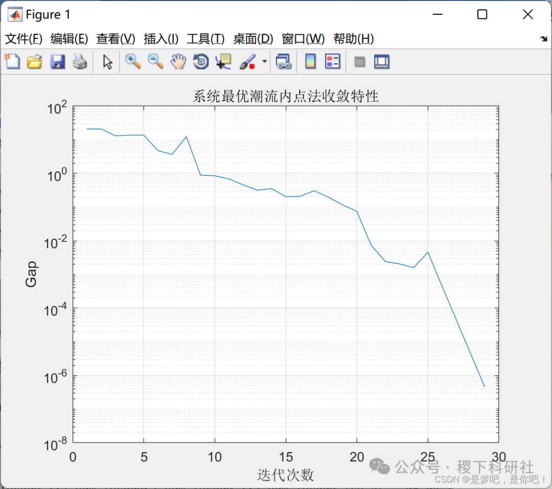

Iterations completed! Time elapsed: 0.186363 seconds. Optimal power flow calculation results:====================================================| Active and Reactive Power Output |==================================================== Generator Node Active Reactive Fuel No. No. Output Output Cost/$ 1 4 5.5056 1.778 3833.0934 2 5 2.1568 2.6194 3870.1109 Total — 7.6624 4.3974 7703.2043====================================================| Node Voltage Phasors |==================================================== Node Voltage Voltage No. Magnitude Phase Angle 1 0.9 -0.006967 2 1.1 0.404913 3 1.0818 -0.057126 4 1.0697 0.478675 5 1.1 0====================================================| Branch Active Power |==================================================== Branch From To Power No. 1 1 2 -1.6064 2 1 3 0.0064 3 2 3 1.7709 4 2 4 -5.5056 5 3 5 -2.1568>

6 References
Some content in this article is sourced from the internet, and references will be noted. If there are any inaccuracies, please feel free to contact for removal. (The content of the article is for reference only, and the actual results may vary.)
7 Complete Matlab Code Download
For more resources, MATLAB|Simulink|Python resources are available.