What is a Filter?
Various sensor signals carry some noise signals to varying degrees, and filters can better reduce and eliminate noise, restoring the true useful signal. A filter is a circuit that removes or “filters out” specific frequency components. In other words, it separates the frequency spectrum of a signal into components that will pass through and components that will be blocked. If you do not have much experience with frequency domain analysis, you may still be unsure about what these frequency components are and how they coexist in a signal that cannot have multiple voltage values simultaneously. Let’s look at a brief example that helps clarify this concept. Suppose we have an audio signal consisting of a perfect 5kHz sine wave. We know what a sine wave looks like in the time domain, and in the frequency domain, we only see a frequency “spike” at 5kHz. Now let’s assume we activate a 500kHz oscillator, introducing high-frequency noise into the audio signal. The signal seen on the oscilloscope is still just a sequence of voltage values, but the signal will look different because its time-domain variation must now reflect both the 5kHz sine wave and the fluctuations of the high-frequency noise. However, in the frequency domain, the sine wave and noise exist as separate frequency components within a single signal. The sine wave and noise occupy different parts of the signal’s frequency domain representation, which means we can filter out the noise by routing the signal through a circuit that passes low frequencies and blocks high frequencies. The distribution of the different parts of the frequency domain for the sine wave and noise signal is shown below.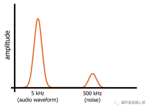
Types of Filters
Filters can be categorized into broad categories that correspond to the general characteristics of the filter’s frequency response. If a filter passes low frequencies and blocks high frequencies, it is called a low-pass filter; if it blocks low frequencies and passes high frequencies, it is a high-pass filter. There are also band-pass filters, which only pass a relatively narrow range of frequencies, and band-stop filters, which only block a relatively narrow range of frequencies. The frequency domain representations of various filters are shown in the figure below.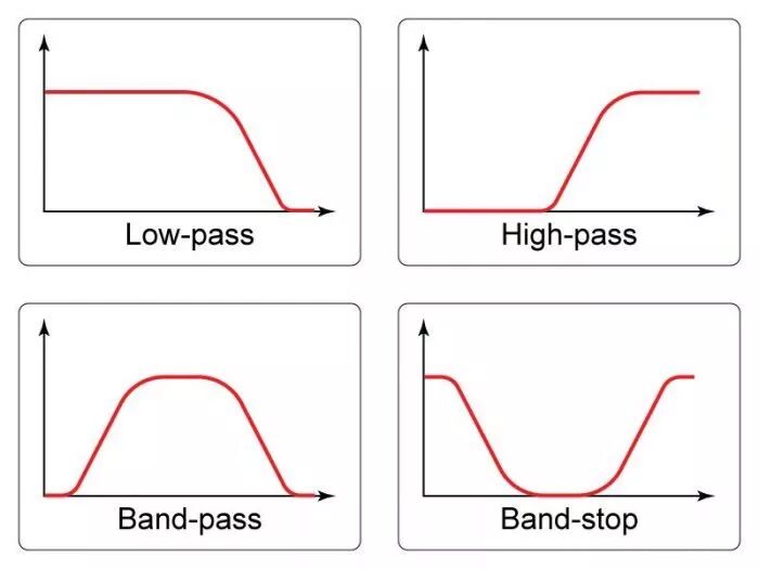 Filters can also be classified based on the type of components used to implement the circuit. Passive filters use resistors, capacitors, and inductors, which do not have the ability to provide amplification, so passive filters can only maintain or reduce the amplitude of the input signal. On the other hand, active filters can filter signals and apply gain because they include active components such as transistors or operational amplifiers, as shown in the figure below.
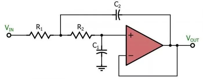 This active low-pass filter is based on the popular Sallen-Key topology. For more details, refer to this article:Sallen-Key Active Filter.
RC Low-Pass Filter
To create a passive low-pass filter, we need to combine resistive elements with reactive elements. In other words, we need a circuit made up of resistors and capacitors or inductors. Theoretically, the resistor-inductor (RL) low-pass topology is comparable to the resistor-capacitor (RC) low-pass topology in terms of filtering capability. However, in practice, the resistor-capacitor scheme is more common, so the remainder of this article will focus on RC low-pass filters. The schematic of an RC low-pass filter is shown below.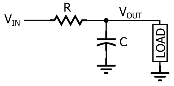 As shown, an RC low-pass response can be generated by placing a resistor in series with the signal path and a capacitor in parallel with the load. In the diagram, the load is a single component, but in actual circuits, it may be more complex, such as an analog-to-digital converter, amplifier, or the input stage of an oscilloscope used to measure the filter’s response. If we recognize that the resistor and capacitor form a voltage divider that is frequency-dependent, we can intuitively analyze the filtering action of the RC low-pass topology. Redrawing the RC low-pass filter to look like a voltage divider, as shown in the figure below.
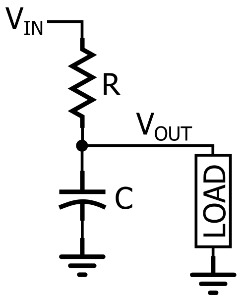 When the frequency of the input signal is low, the impedance of the capacitor is high relative to the impedance of the resistor; therefore, most of the input voltage drops across the capacitor (and across the load in parallel with the capacitor). When the input frequency is higher, the impedance of the capacitor is lower relative to the impedance of the resistor, which means the voltage across the resistor decreases, and less voltage is transmitted to the load. Thus, low frequencies pass through while high frequencies are blocked. This qualitative explanation of the RC low-pass function is an important first step, but it is not very useful when we need to actually design a circuit, as the terms “high frequency” and “low frequency” are very vague. Engineers need to create circuits that pass and block specific frequencies. For example, in the audio system mentioned above, we want to preserve the 5kHz signal while suppressing the 500kHz signal. This means we need a filter that transitions from passing frequencies at 5kHz to blocking frequencies at 500kHz.RC Filter Cutoff Frequency The frequency range where the filter does not cause significant attenuation is called the passband, while the frequency range where the filter does cause significant attenuation is called the stopband. Analog filters, such as RC low-pass filters, always transition gradually from the passband to the stopband. This means there is no single frequency at which the filter stops passing signals and starts blocking signals. However, engineers need a convenient and concise way to summarize the filter’s frequency response, which is where the concept of cutoff frequency comes into play.When you look at the frequency response graph of an RC filter, you will notice that the term “cutoff frequency” is not very accurate. The image of the signal spectrum being “cut” in half, where one half is retained and the other is discarded, is not applicable because the attenuation gradually increases as the frequency moves from below the cutoff point to above the cutoff value. The cutoff frequency of an RC low-pass filter is actually the frequency at which the input signal amplitude is reduced by 3dB (the choice of this value is because a 3dB reduction in amplitude corresponds to a 50% reduction in power). Therefore, the cutoff frequency is also referred to as the -3dB frequency, and this name is actually more accurate and informative. The term bandwidth refers to the width of the filter’s passband, which, in the case of a low-pass filter, is equal to the -3dB frequency, as shown in the figure below.
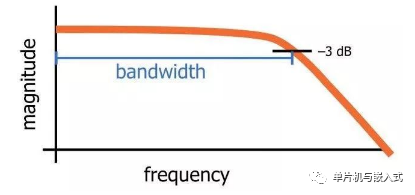 The above figure represents the general characteristics of the frequency response of an RC low-pass filter, where the bandwidth is equal to the -3dB frequency. As mentioned earlier, the low-pass behavior of the RC filter is caused by the interaction between the frequency-independent impedance of the resistor and the frequency-dependent impedance of the capacitor. To determine the details of the filter’s frequency response, we need to mathematically analyze the relationship between the resistance (R) and capacitance (C), and we can also manipulate these values to design a filter that meets precise specifications. The cutoff frequency (fC) of an RC low-pass filter is calculated as follows:
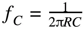 Let’s look at a simple design example. The capacitance value is more restrictive than the resistance value, so we will start with a common capacitance value (e.g., 10nF), and then we will use that formula to determine the required resistance value. The goal is to design a filter that will preserve the 5kHz audio waveform and suppress the 500kHz noise waveform. We will try a cutoff frequency of 100kHz, and we will analyze this filter’s effect on the two frequency components later in the article, using the formula below.
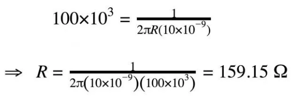 Therefore, a 160Ω resistor combined with a 10nF capacitor will provide us with a filter that is very close to the desired frequency response.
Visualizing Filter Response
The most convenient way to evaluate the filter’s effect on the signal is to examine the graph of the filter’s frequency response. These graphs are commonly referred to as Bode plots, with amplitude (in decibels) on the vertical axis and frequency on the horizontal axis; the horizontal axis typically has a logarithmic scale, making the physical distance between 1Hz and 10Hz the same as that between 10Hz and 100Hz, and between 100Hz and 1kHz, etc. This configuration allows us to quickly and accurately assess the filter’s behavior over a wide frequency range.Below is an example of a frequency response graph.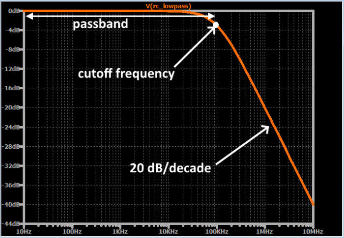 Each point on the curve represents the amplitude that the output signal will have if the input signal’s amplitude is 1V and the frequency equals the corresponding value on the horizontal axis. For example, when the input frequency is 1MHz, the output amplitude (assuming the input amplitude is 1V) will be 0.1V (because -20dB corresponds to a tenfold reduction factor). As you spend more time using filter circuits, the general shape of this frequency response curve will become very familiar. The curve in the passband is almost completely flat, and then as the input frequency approaches the cutoff frequency, it begins to drop off more steeply. Eventually, the rate of change of attenuation (called the roll-off) stabilizes at 20dB/decade—that is, for every tenfold increase in input frequency, the output signal’s amplitude decreases by 20dB.
Evaluating Low-Pass Filter Performance
If we carefully plot the frequency response of the filter we designed earlier in this article, we will see that the amplitude response at 5kHz is essentially 0dB (i.e., almost no attenuation), while the amplitude response at 500kHz is about -14dB (corresponding to a gain of 0.2). These values are consistent with the calculations we performed in the previous section. Since RC filters always transition gradually from the passband to the stopband, and because attenuation never reaches infinity, we cannot design a “perfect” filter—that is, a filter that has no effect on the sine wave and completely eliminates noise. Instead, we always need to make trade-offs. If we move the cutoff frequency closer to 5kHz, we will have more noise attenuation, but the sine wave we want to send to the speaker will also be attenuated more. If we move the cutoff frequency closer to 500kHz, the attenuation at the sine wave frequency will decrease, but the attenuation at the noise frequency will also decrease. Previously, we discussed how filters modify the amplitudes of various frequency components in a signal. However, in addition to amplitude effects, reactive circuit elements always introduce phase shifts.
Phase Shift in Low-Pass Filters
The concept of phase refers to the value of a periodic signal at a specific moment within its cycle. Therefore, when we say that a circuit causes a phase shift, we mean that it creates a deviation between the input and output signals: the input and output signals no longer start and end their cycles at the same time. The phase shift value (e.g., 45° or 90°) indicates the amount of deviation produced. Each reactive element in the circuit introduces a 90° phase shift, but this phase shift does not occur simultaneously. The phase of the output signal gradually changes with increasing input frequency, just like the amplitude of the output signal. The RC low-pass filter has one reactive element (the capacitor), and thus the circuit will ultimately introduce a 90° phase shift as well. As with amplitude response, the phase response can be most easily evaluated by examining a curve that represents logarithmic frequency on the horizontal axis. The following description represents a general pattern, and the figure below can provide further details.
- The phase shift starts at 0°
- The phase shift gradually increases until it reaches 45° at the cutoff frequency, during which the rate of change gradually increases
- After the cutoff frequency, the phase shift continues to increase, but the rate of change gradually decreases
- As the phase shift approaches 90°, the rate of change becomes very small
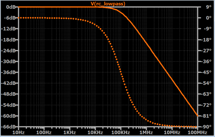 The solid line represents the amplitude response, while the dashed line represents the phase response. The cutoff frequency is 100kHz. Note that the phase shift below the cutoff frequency is 45°.
Second-Order Low-Pass Filters
So far, we have assumed that the RC low-pass filter consists of one resistor and one capacitor. This configuration is a first-order filter. The “order” of a passive filter is determined by the number of reactive elements (i.e., capacitors or inductors) in the circuit. Higher-order filters have more reactive elements, resulting in more phase shift and steeper roll-off, which is the primary motivation for increasing the order of the filter. Adding a reactive element to the filter, such as going from first-order to second-order or from second-order to third-order, can increase the maximum roll-off by 20dB/decade. Second-order filters are typically built around a resonant circuit made up of inductors and capacitors, a topology known as RLC (Resistor-Inductor-Capacitor). However, second-order RC filters can also be created. As shown in the figure below, all we need to do is cascade two first-order RC filters together. While this topology will certainly produce a second-order response, it is not widely used, and its frequency response is generally not as good as that of second-order active filters or second-order RLC filters.
Frequency Response of Second-Order RC Filters
We can attempt to design a first-order filter based on the desired cutoff frequency and then select two of them to connect in series, thus forming a second-order RC low-pass filter. This does indeed allow the filter to exhibit a similar overall frequency response, with a maximum roll-off of 40dB/decade instead of 20dB/decade. However, if we look more closely at the response, we will find that the -3dB frequency appears to be lower. The behavior of the second-order RC filter does not meet expectations because the two filter stages are not independent, and thus we cannot simply connect the two filters together and analyze the circuit as a first-order low-pass filter superimposed with another identical first-order low-pass filter. Furthermore, even if we insert a buffer between the two stages, allowing the first-order RC and second-order RC to function as independent filters, the attenuation at the original cutoff frequency will be 6dB instead of 3dB. This is precisely because the two stages operate independently. The first filter has 3dB of attenuation at the cutoff frequency, and the second filter adds another 3dB of attenuation, as shown in the figure below.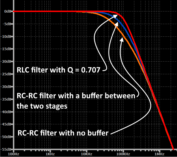 The fundamental limitation of the second-order RC low-pass filter is that designers cannot fine-tune the transition from passband to stopband by adjusting the filter’s Q factor; this parameter indicates the degree of damping in the frequency response. If two identical RC low-pass filters are cascaded, the overall transfer function corresponds to a second-order response, but the Q factor is always 0.5. When Q=0.5, the filter is at the boundary of being over-damped, which causes the frequency response to “droop” in the transition region. Second-order active filters and second-order resonant filters do not have this limitation; designers can control the Q factor, allowing them to fine-tune the frequency response in the transition region.
Conclusion
All electrical signals are a mix of desired frequency components and unwanted frequency components. Unwanted frequency components are often caused by noise and interference, and in some cases, they can negatively impact system performance. Filters are circuits that respond differently to different parts of the signal spectrum. Low-pass filters are designed to allow low-frequency components to pass while blocking high-frequency components. The cutoff frequency of a low-pass filter indicates the frequency region where the filter transitions from low attenuation to significant attenuation. The output voltage of an RC low-pass filter can be calculated by viewing the circuit as a voltage divider made up of (frequency-independent) resistance and (frequency-dependent) reactance. A curve graph of amplitude (in dB on the vertical axis) versus logarithmic frequency (in Hz on the horizontal axis) is a convenient and effective way to examine the theoretical behavior of the filter, and a graph of phase versus logarithmic frequency can also be used to determine the amount of phase shift that will be applied to the input signal. Second-order filters have steeper roll-offs; this second-order response is useful when the signal cannot provide wideband separation between the desired frequency components and the unwanted frequency components. A second-order RC low-pass filter can be created by building two identical first-order RC low-pass filters and then connecting the output of one to the input of the other, but ultimately the overall -3dB frequency will be lower than expected.