The program is open, complete, and free.
Program version: MATLAB 2010
Debugging this program took about 4 hours, and it was done in a hurry. There may be some issues, and I welcome your feedback.
The simulation program constructs a complete electric vehicle model, including three main modules: vehicle basic parameters, battery system, and motor system. The program simulates the vehicle’s driving process under the NEDC standard conditions, calculating air resistance, rolling resistance, and acceleration resistance during the driving process through precise physical formulas, thereby determining the power demand of the motor.
In the battery model section, the program considers both discharge and regenerative braking modes, calculating the battery’s current, voltage, and state of charge (SOC) in real-time. Through the energy recovery system, the electric vehicle can effectively recover braking energy, enhancing its range.
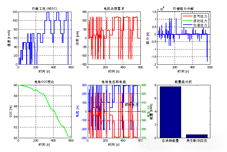
The program visualizes results, including speed curves, power demand, resistance analysis, SOC changes, and six subplots that intuitively display the vehicle’s operating status. Through this simulation, we can calculate key performance indicators: energy consumption per 100 kilometers, total energy consumption, and average system efficiency.
|
%% Electric Vehicle Power System Simulation and Analysis % Version: 1.0 % Applicable to: MATLAB 2010 clear; close all; clc; %% 1. Vehicle Parameter Definition fprintf(‘=== Electric Vehicle Power System Parameter Settings ===\n’); % Vehicle basic parameters vehicle.mass = 1500; % Vehicle mass [kg] vehicle.frontal_area = 2.2; % Frontal area [m²] vehicle.drag_coefficient = 0.28; % Drag coefficient vehicle.rolling_resistance = 0.015; % Rolling resistance coefficient vehicle.wheel_radius = 0.3; % Wheel radius [m] vehicle.transmission_efficiency = 0.95; % Transmission efficiency % Battery parameters battery.capacity = 60; % Battery capacity [kWh] battery.voltage = 400; % Battery voltage [V] battery.initial_soc = 0.9; % Initial SOC battery.internal_resistance = 0.1; % Internal resistance [Ω] % Motor parameters motor.max_power = 120; % Maximum power [kW] motor.max_torque = 300; % Maximum torque [Nm] motor.efficiency_map = [0.85, 0.90, 0.92, 0.91, 0.88; % Efficiency mapping matrix 0.88, 0.92, 0.94, 0.93, 0.90; 0.85, 0.91, 0.93, 0.92, 0.89; 0.82, 0.88, 0.90, 0.89, 0.86]; %% 2. Driving Condition Generation fprintf(‘=== Generating Standard Driving Conditions ===\n’); % Time parameters sim_time = 600; % Simulation time [s] dt = 1; % Time step [s] t = 0:dt:sim_time; % Generate NEDC conditions (inline function to avoid file separation issues) speed_profile = zeros(size(t)); for i = 1:length(t) if t(i) <= 195 % Urban cycle if t(i) <= 15 speed_profile(i) = 0; elseif t(i) <= 23 speed_profile(i) = 15; elseif t(i) <= 28 speed_profile(i) = 0; elseif t(i) <= 44 speed_profile(i) = 32; elseif t(i) <= 50 speed_profile(i) = 10; elseif t(i) <= 56 speed_profile(i) = 50; elseif t(i) <= 61 speed_profile(i) = 35; elseif t(i) <= 86 speed_profile(i) = 50; elseif t(i) <= 93 speed_profile(i) = 35; elseif t(i) <= 98 speed_profile(i) = 0; elseif t(i) <= 108 speed_profile(i) = 50; elseif t(i) <= 113 speed_profile(i) = 70; elseif t(i) <= 121 speed_profile(i) = 50; elseif t(i) <= 126 speed_profile(i) = 35; elseif t(i) <= 134 speed_profile(i) = 50; elseif t(i) <= 139 speed_profile(i) = 0; elseif t(i) <= 145 speed_profile(i) = 70; elseif t(i) <= 151 speed_profile(i) = 50; elseif t(i) <= 156 speed_profile(i) = 0; elseif t(i) <= 178 speed_profile(i) = 70; elseif t(i) <= 185 speed_profile(i) = 50; elseif t(i) <= 190 speed_profile(i) = 35; else speed_profile(i) = 0; end else % Suburban cycle cycle_time = mod(t(i)-195, 400); if cycle_time <= 20 speed_profile(i) = 0; elseif cycle_time <= 55 speed_profile(i) = 70; elseif cycle_time <= 85 speed_profile(i) = 50; elseif cycle_time <= 105 speed_profile(i) = 70; elseif cycle_time <= 130 speed_profile(i) = 100; elseif cycle_time <= 155 speed_profile(i) = 120; elseif cycle_time <= 175 speed_profile(i) = 100; elseif cycle_time <= 195 speed_profile(i) = 70; elseif cycle_time <= 205 speed_profile(i) = 50; elseif cycle_time <= 215 speed_profile(i) = 70; elseif cycle_time <= 240 speed_profile(i) = 100; elseif cycle_time <= 265 speed_profile(i) = 120; elseif cycle_time <= 285 speed_profile(i) = 100; elseif cycle_time <= 305 speed_profile(i) = 70; elseif cycle_time <= 315 speed_profile(i) = 50; elseif cycle_time <= 325 speed_profile(i) = 70; elseif cycle_time <= 350 speed_profile(i) = 100; elseif cycle_time <= 370 speed_profile(i) = 120; else speed_profile(i) = 0; end end end % Calculate acceleration acceleration = zeros(size(speed_profile)); if length(speed_profile) > 1 acceleration(2:end) = diff(speed_profile) / dt; end %% 3. Power Demand Calculation fprintf(‘=== Calculating Vehicle Power Demand ===\n’); % Air resistance air_resistance = 0.5 * 1.225 * vehicle.drag_coefficient * … vehicle.frontal_area * speed_profile.^2; % Rolling resistance rolling_resistance = vehicle.mass * 9.81 * vehicle.rolling_resistance * … cos(0); % Assuming level road % Acceleration resistance acceleration_resistance = vehicle.mass * acceleration; % Total driving resistance total_resistance = air_resistance + rolling_resistance + acceleration_resistance; % Power demand calculation wheel_torque = total_resistance * vehicle.wheel_radius; wheel_power = wheel_torque .* (speed_profile / 3.6) / vehicle.wheel_radius; motor_power_demand = wheel_power / vehicle.transmission_efficiency; % Limit within the motor’s maximum power range motor_power_demand = min(motor_power_demand, motor.max_power * 1000); motor_power_demand = max(motor_power_demand, -motor.max_power * 1000); % Regenerative braking %% 4. Battery Model Simulation fprintf(‘=== Battery System Simulation ===\n’); % Initialize SOC array soc = zeros(size(t)); soc(1) = battery.initial_soc; % Battery current and voltage calculation battery_current = zeros(size(t)); battery_voltage = zeros(size(t)); for i = 1:length(t) if motor_power_demand(i) > 0 % Discharge mode battery_current(i) = motor_power_demand(i) / battery.voltage; battery_voltage(i) = battery.voltage – battery_current(i) * battery.internal_resistance; else % Regenerative braking charging mode (efficiency 0.7) battery_current(i) = motor_power_demand(i) * 0.7 / battery.voltage; battery_voltage(i) = battery.voltage – battery_current(i) * battery.internal_resistance; end % SOC update if i < length(t) energy_consumed = battery_current(i) * battery_voltage(i) * dt / 3600; % [Wh] soc(i+1) = soc(i) – energy_consumed / (battery.capacity * 1000); soc(i+1) = max(0, min(1, soc(i+1))); % SOC limited between 0-1 end end %% 5. Performance Indicator Calculation fprintf(‘=== Calculating Performance Indicators ===\n’); % Total driving distance distance = trapz(t, speed_profile/3.6); % [km] % Energy consumption total_energy_consumed = (battery.initial_soc – soc(end)) * battery.capacity; % [kWh] % Avoid division by zero if distance > 0 energy_consumption = total_energy_consumed / distance * 100; % [kWh/100km] else energy_consumption = 0; end % Average efficiency positive_power_indices = find(motor_power_demand > 0); if ~isempty(positive_power_indices) average_efficiency = mean(motor_power_demand(positive_power_indices) ./ … (battery_current(positive_power_indices) .* … battery_voltage(positive_power_indices))); else average_efficiency = 0; end %% 6. Result Visualization fprintf(‘=== Generating Simulation Result Charts ===\n’); figure(‘Position’, [100, 100, 1200, 800]); % Subplot 1: Driving conditions subplot(2,3,1); plot(t, speed_profile, ‘b-‘, ‘LineWidth’, 2); xlabel(‘Time [s]’); ylabel(‘Speed [km/h]’); title(‘Driving Conditions (NEDC)’); grid on; % Subplot 2: Power demand subplot(2,3,2); plot(t, motor_power_demand/1000, ‘r-‘, ‘LineWidth’, 2); xlabel(‘Time [s]’); ylabel(‘Power [kW]’); title(‘Motor Power Demand’); grid on; % Subplot 3: Resistance analysis subplot(2,3,3); plot(t, air_resistance, ‘r-‘, t, rolling_resistance*ones(size(t)), ‘g-‘, … t, acceleration_resistance, ‘b-‘, ‘LineWidth’, 2); xlabel(‘Time [s]’); ylabel(‘Resistance [N]’); title(‘Driving Resistance Breakdown’); legend(‘Air Resistance’, ‘Rolling Resistance’, ‘Acceleration Resistance’); grid on; % Subplot 4: SOC changes subplot(2,3,4); plot(t, soc*100, ‘g-‘, ‘LineWidth’, 2); xlabel(‘Time [s]’); ylabel(‘SOC [%]’); title(‘Battery SOC Changes’); grid on; % Subplot 5: Battery parameters – using plotyy instead of yyaxis (compatible with 2010 version) subplot(2,3,5); [ax, h1, h2] = plotyy(t, battery_current, t, battery_voltage); set(h1, ‘LineWidth’, 2, ‘Color’, ‘b’); set(h2, ‘LineWidth’, 2, ‘Color’, ‘r’); ylabel(ax(1), ‘Current [A]’); ylabel(ax(2), ‘Voltage [V]’); xlabel(‘Time [s]’); title(‘Battery Voltage and Current’); grid on; % Add rated voltage reference line (replace yline) hold(ax(2), ‘on’); plot(ax(2), t, battery.voltage * ones(size(t)), ‘k–‘, ‘LineWidth’, 1); text(t(end)*0.7, battery.voltage*1.02, ‘Rated Voltage’, ‘Parent’, ax(2)); hold(ax(2), ‘off’); % Subplot 6: Energy flow subplot(2,3,6); regenerative_indices = find(motor_power_demand < 0); if ~isempty(regenerative_indices) regenerative_energy = abs(sum(motor_power_demand(regenerative_indices)) * dt / 3600 / 1000); % kWh else regenerative_energy = 0; end labels = {‘Total Consumed Energy’, ‘Regenerative Braking Recovery’}; values = [total_energy_consumed, regenerative_energy]; bar(values); set(gca, ‘XTickLabel’, labels); ylabel(‘Energy [kWh]’); title(‘Energy Flow Analysis’); %% 7. Result Display fprintf(‘\n=== Simulation Result Summary ===\n’); fprintf(‘Total driving distance: %.2f km\n’, distance); fprintf(‘Total energy consumption: %.2f kWh\n’, total_energy_consumed); fprintf(‘Energy consumption rate: %.2f kWh/100km\n’, energy_consumption); fprintf(‘Final SOC: %.1f%%\n’, soc(end)*100); fprintf(‘Average efficiency: %.1f%%\n’, average_efficiency*100); fprintf(‘Regenerative braking recovery energy: %.2f kWh\n’, regenerative_energy); |
 |
Everyone is welcome to share!!!