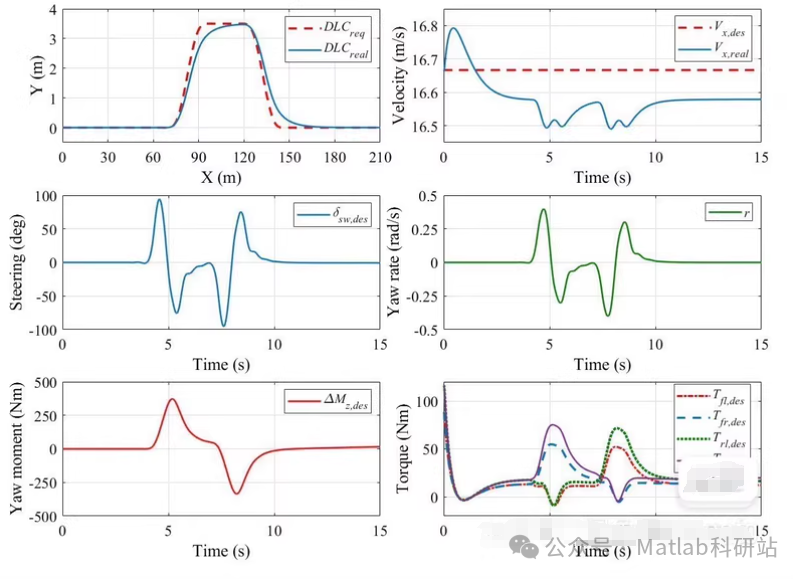
Trajectory Tracking and Stability Control of Distributed Drive Electric Vehicles Based on MATLAB

Trajectory Tracking and Stability Control of Distributed Drive Electric Vehicles Based on MATLAB① The upper layer of the controller uses Model Predictive Control (MPC) to determine the front wheel steering angle (δ) and additional yaw moment (ΔMz), achieving trajectory tracking control and stability control for autonomous distributed electric vehicles in a Double Lane Change (DLC) scenario.② The lower layer of the controller is based on Quadratic Programming (QP) for torque optimization distribution.③ This approach is very helpful for learning the control and torque distribution of distributed drive vehicles.

Trajectory Tracking and Stability Control of Distributed Drive Electric Vehicles Based on MATLAB The following text and example code are for reference only.

Article Directory

📌 System Structure Overview
✅ Vehicle Dynamics Model (Bicycle Model)
🧠 Upper Layer Controller: Model Predictive Control (MPC)

Objective Function Design

🧠 Lower Layer Controller: Quadratic Programming (QP) Allocator
📈 Reference Trajectory Generation: Double Lane Change (DLC)
📊 Suggested Structure for Simulink Modules
📦 Example Simulink Structure Diagram
🧪 Operation Process Description
📚 Recommended References

The following is a complete implementation plan for Trajectory Tracking and Stability Control of Distributed Drive Electric Vehicles based on MATLAB/Simulink, covering:

Upper Layer Controller:Model Predictive Control (MPC)

Determining the front wheel steering angle δ and additional yaw moment ΔMz

Lower Layer Controller:Quadratic Programming (QP) Optimization Distribution

Rationally distributing the desired yaw moment and longitudinal force to the four wheels

Control Scenario:Double Lane Change (DLC)

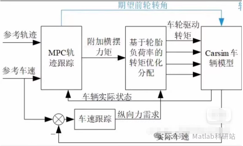
📌 System Structure Overview

[Reference Trajectory] → [MPC Controller] → [QP Allocator] → [4 Wheel Torque Outputs]
                            ↑
                       [Vehicle State Feedback]

✅ Vehicle Dynamics Model (Bicycle Model)

% Single-track model (simplified vehicle kinematics)
function dx = vehicle_model(x, u, params)
% x = [x; y; psi; vx; vy; r]
% u = [delta; Fx_front; Fx_rear; Mz]

    m = params.m;
    Iz = params.Iz;
    lf = params.lf;
    lr = params.lr;
    vx = x(4);
    vy = x(5);
    r = x(6);

    beta = atan2(vy, vx); % Side slip angle
    Fy_f = -params.Cf * (beta + lf*r/vx - u(1)); % Front wheel lateral force
    Fy_r = -params.Cr * (beta - lr*r/vx); % Rear wheel lateral force

    dxdt = [
        vx*cos(psi) - vy*sin(psi);
        vx*sin(psi) + vy*cos(psi);
        r;
        (u(2) + u(3))/m - r*vy;
        (Fy_f + Fy_r)/m + r*vx;
        (lf*Fy_f - lr*Fy_r + u(4))/Iz
    ];
end

🧠 Upper Layer Controller: Model Predictive Control (MPC)

Objective Function Design

Minimize trajectory error (lateral displacement, heading angle) while constraining input variations.

% Set MPC parameters
N = 10; % Prediction horizon
Q = diag([10, 10, 1]); % Weights for lateral error, heading error, speed error
R = diag([0.1, 0.1]); % Input weights (front wheel steering angle, yaw moment)

% Construct MPC problem (using MATLAB Optimization Toolbox)
mpcobj = mpc(vehicle_ss, Ts, N, N);
setWeights(mpcobj, 'MV', R(1), 'MVRate', 0.01);
setWeights(mpcobj, 'Output', Q);
setConstraints(mpcobj, [], [], [-0.5; -500], [0.5; 500]); % δ ∈ [-0.5, 0.5], ΔMz ∈ [-500, 500]

Note: You can also use ACADO ToolKit or CasADi to implement a more efficient nonlinear MPC.

🧠 Lower Layer Controller: Quadratic Programming (QP) Allocator

Distributes the total torque and longitudinal force output from MPC to the four wheels, satisfying tire force ellipse constraints.

% Define variables: drive forces for four wheels Fx_i
% Constraints:
%     Fx_fl + Fx_fr + Fx_rl + Fx_rr = F_total
%     lf*(Fx_fl + Fx_fr) - lr*(Fx_rl + Fx_rr) = ΔMz
%     Fx_i >= 0 (only drive)
%     Fx_i <= μ*N_i (friction limit)

% Construct QP problem
H = eye(4); % Minimize the sum of squares of drive forces (smooth distribution)
f = zeros(4, 1);

Aeq = [
    1 1 1 1; % Total drive force
    lf lf -lr -lr % Yaw moment
];
b_eq = [F_total; delta_Mz];

lb = [0; 0; 0; 0]; % Cannot be negative when driving
ub = [mu*N_fl; mu*N_fr; mu*N_rl; mu*N_rr]; % Friction limit

% Solve using quadprog
Fx_opt = quadprog(H, f, [], [], Aeq, b_eq, lb, ub);

📈 Reference Trajectory Generation: Double Lane Change (DLC)

% Generate DLC reference trajectory
t = 0:Ts:T_sim;
x_ref = 20 * t; % Longitudinal displacement
y_ref = 1.75 * erf(t/1.2); % Lateral displacement (erf function simulates smooth lane change)

ref_traj = [x_ref' y_ref'];

📊 Suggested Structure for Simulink Modules

Module	Function
Reference Path Generator	Generates DLC reference trajectory
MPC Controller	Model Predictive Controller
QP Allocator	Torque Optimization Allocator
Vehicle Dynamics	Complete vehicle dynamics model (can use Vehicle Dynamics Blockset)
Tire Force Model	Includes tire mechanics constraints
Scope & Visualization	Displays trajectory tracking results

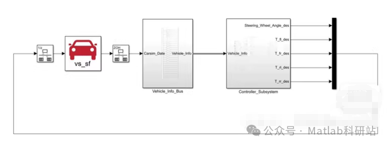
📦 Example Simulink Structure Diagram

[Reference Trajectory] --> [MPC Controller] --> [QP Allocator] --> [Wheel Torque Inputs]
                                                  ↑
                                             [Vehicle Feedback]

🧪 Operation Process Description

Initialize vehicle state, parameters, and reference trajectory
In each control cycle:

Obtain current vehicle state
Use MPC to calculate optimal δ and ΔMz
Distribute to obtain drive forces for the four wheels via QP
Input to the complete vehicle model for simulation
Update state and plot results

📚 Recommended References

“Model Predictive Control for Autonomous and Electric Vehicles”
IEEE Paper:“Torque Vectoring and Yaw Control for Electric Vehicles Using Quadratic Programming”
MATLAB Official Examples:

mpc_car example
quadprog function documentation

Open Source Projects on GitHub:

ACADO for MPC
Apollo Auto (Baidu Autonomous Driving System)