Original link: http://tecdat.cn/?p=24103
This example illustrates how to perform Bayesian inference using a logistic regression model (click “Read the original” at the end of the article to obtain the complete code data).
Statistical inference is typically based on Maximum Likelihood Estimation (MLE). MLE selects parameters that maximize the likelihood of the data, which is a natural approach. In MLE, parameters are assumed to be unknown but fixed values, and calculations are performed under a certain confidence level. In Bayesian statistics, probabilities are used to quantify the uncertainty of unknown parameters, treating them as random variables.
Related Video
Bayesian Inference
Bayesian inference is the process of analyzing statistical models by combining prior knowledge about the model or model parameters. The foundation of this inference is Bayes’ theorem:

For example, suppose we have normally distributed observations
where sigma is known, and the prior distribution of theta is
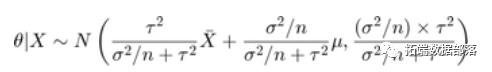
In this formula, mu and tau (sometimes referred to as hyperparameters) are also known. If we observe <span>X</span> with <span>n</span> samples, we can obtain the posterior distribution of theta
The following figure shows the prior, likelihood, and posterior of theta.
y = norpdf(thta, posMan,psSD);
plot(theta'-', theta,'--', theta,'-.')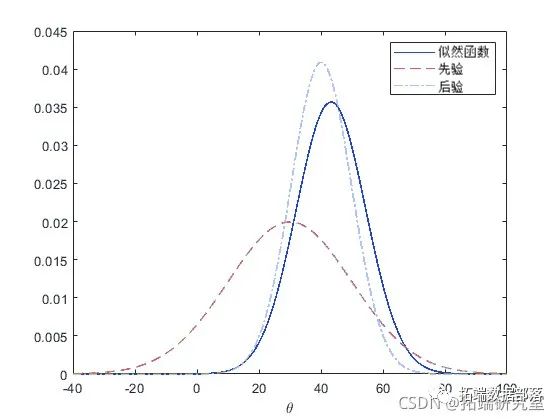
Automotive Experimental Data
In some simple problems, such as the previous example of normal mean inference, it is easy to compute the posterior distribution in closed form. However, in general problems involving non-conjugate priors, the posterior distribution is difficult or impossible to compute analytically. We will use logistic regression as an example. This example includes an experiment to help model the failure rate of cars of different weights in mileage tests. The data includes observations such as the weight of the tested cars, the number of cars, and the number of failures. We use a set of transformed weights to reduce the correlation in the estimation of regression parameters.
% A set of car weights
% Number of cars tested at each weight
[48 42 31 34 31 21 23 23 21 16 17 21]';
% Number of cars with poor mpg performance at each weight
[1 2 0 3 8 8 14 17 19 15 17 21]';
Logistic Regression Model
Logistic regression (a special case of generalized linear models) is suitable for these data because the dependent variable follows a binomial distribution. The logistic regression model can be written as:
where X is the design matrix, and b is the vector containing the model parameters. We can express this equation as:
@(b,x) exp(b(1)+b(2).*x)./(1+exp(b(1)+b(2).*x));If you have some prior knowledge or already possess some non-informative priors, you can specify the prior probability distribution for the model parameters. For example, in this example, we use normal priors to represent the intercept <span>b1</span> and slope <span>b2</span><code><span>, that is</span>
@(b1) normpdf(b1,0,20); % Prior for intercept.
@(b2) normpdf(b2,0,20); % Prior for slope.
According to Bayes’ theorem, the joint posterior distribution of the model parameters is proportional to the product of the likelihood and the prior.
Note that the normalization constant of the posterior in this model is difficult to analyze. However, even without knowing the normalization constant, if you know the approximate range of the model parameters, you can visualize the posterior distribution.
msh(b2,b1,sipot)
view(-10,30)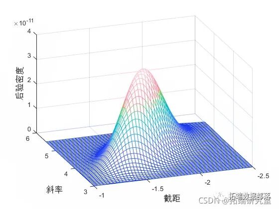
This posterior stretches along the diagonal of the parameter space, indicating that (after observing the data) we believe the parameters are correlated. This is interesting because we assumed they were independent before collecting any data. The correlation arises from the combination of our prior distribution and the likelihood function.
Click the title to check previous content

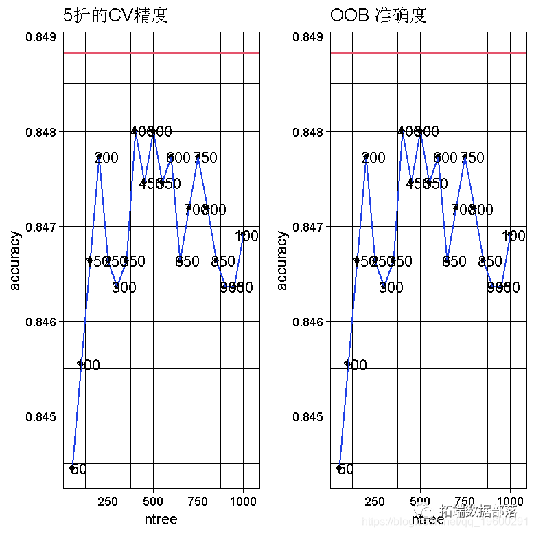
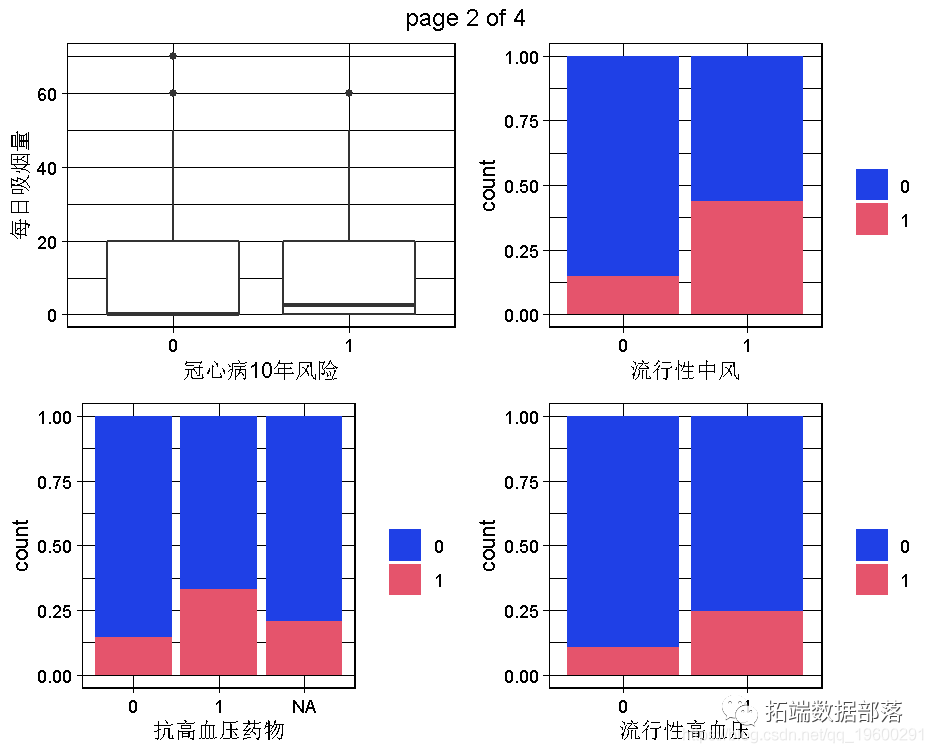
R language random forest RandomForest, logistic regression Logistic prediction of heart disease data and visualization analysis

Swipe left to see more
01
02
03
04
Slice Sampling
The Monte Carlo method is often used to summarize posterior distributions in Bayesian data analysis. The idea is that even if you cannot compute the posterior distribution analytically, you can generate random samples from the distribution and use these random values to estimate posterior distribution statistics, such as posterior mean, median, standard deviation, etc. Slice sampling is an algorithm used to sample from distributions with arbitrary density functions, known to have at most one proportionality constant – which is exactly what is needed to sample from complex posterior distributions with unknown normalization constants. This algorithm does not generate independent samples but generates a Markov chain whose stationary distribution is the target distribution. Therefore, the slice sampler is a Markov Chain Monte Carlo (MCMC) algorithm. However, it differs from other well-known MCMC algorithms because it only requires the specification of the scaled posterior, without needing a proposal distribution or marginal distribution.
This example illustrates how to use the slice sampler as part of the Bayesian analysis of the mileage test logistic regression model, including generating random samples from the posterior distribution of model parameters, analyzing the output of the sampler, and making inferences about the model parameters. The first step is to generate random samples.
sliesmle(inial,nsapes,'pdf');Analysis of Sampler Output
After obtaining random samples from slice sampling, it is important to investigate issues such as convergence and mixing to determine whether it is reasonable to consider the samples as a set of random realizations from the target posterior distribution. Observing the marginal trace plots is the simplest way to check the output.
plot(trace(:,1))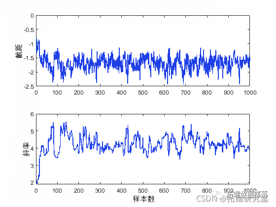
From these plots, it is evident that the influence of the initial values of the parameters persists for a while (about 50 samples) before dissipating as the process stabilizes.
Checking convergence by calculating statistics (e.g., mean, median, or standard deviation) using a moving window is also helpful. This can produce smoother plots than the original sample traces and make it easier to identify and understand any non-stationarity.
mvag = fier( (1/50)*os(50,1), 1, tace);
plot(moav(:,1))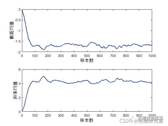
Since these are moving averages based on windows containing 50 iterations, the first 50 values cannot be compared with the other values in the plot. However, the other values in each plot seem to confirm that the posterior mean of the parameters converges to a stationary distribution after about 100 iterations. It is also evident that these two parameters are correlated with each other, consistent with the previous posterior density plots.
Since the burn-in period represents samples that cannot reasonably be considered random realizations from the target distribution, it is not advisable to use the first 50 or so values output by the slice sampler. You can simply delete these output rows, but you can also specify a “burn-in” period. This approach is convenient when the appropriate burn-in length is known (possibly from previous runs).
slcsapl(inial,nsmes,'pf',pot, ..'brin',50);
plot(trace(:,1))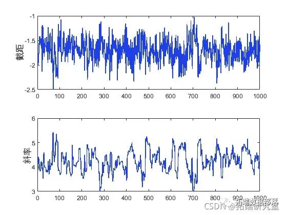
These trace plots show no signs of non-stationarity, indicating that the burn-in period has been completed.
However, it is also important to understand another aspect of the trace plots. While the trace of the intercept appears to be high-frequency noise, the trace of the slope seems to have low-frequency components, indicating autocorrelation between adjacent iteration values. While it is also possible to calculate means from this autocorrelated sample, we typically reduce storage requirements by simply removing redundant data from the sample. If it simultaneously eliminates autocorrelation, we can also treat this data as independent value samples. For example, you can dilute the sample by only retaining every 10th, 20th, 30th, etc. value.
sceampe(...
                                                'brin'50,'tin',10);
To check the effect of this dilution, you can estimate the sample autocorrelation function based on the traces and use them to check whether the sample mixes quickly.
fftetendtrce,'cnsant');
F .* coj(F);

for i = 1:2
   lineles =  stem(:20, F(:i)  'filled' , 'o');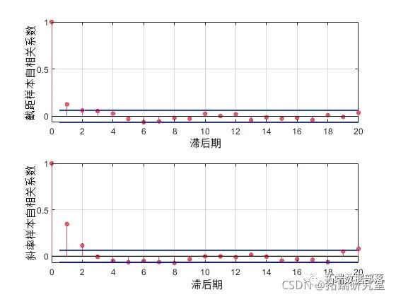
The first lagged autocorrelation value is evident for the intercept parameter and even more so for the slope parameter. We can repeat sampling with a larger dilution parameter to further reduce correlation. But for the purposes of this example, we will continue using the current sample.
Inference of Model Parameters
As expected, the sample histogram simulates the posterior density plot.
hist(rce,[25,25]);
view(-10,30)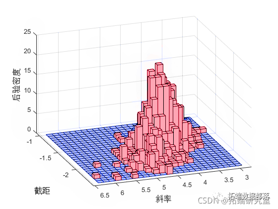
You can summarize the marginal distribution properties of the posterior samples using histograms or kernel density estimates.
kdeiy(rae(:2))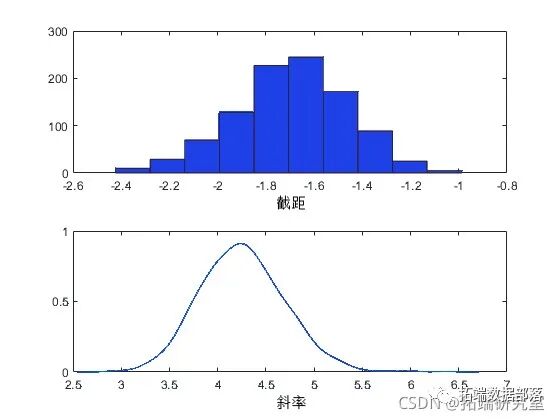
You can also calculate descriptive statistics, such as the posterior mean or percentiles of the random samples. To determine whether the sample size is sufficient to achieve the desired accuracy, it is helpful to view the required trajectory statistics as a function of the sample size.
csu= csm(rae);

plot(csm(:,1)'./(1:sals))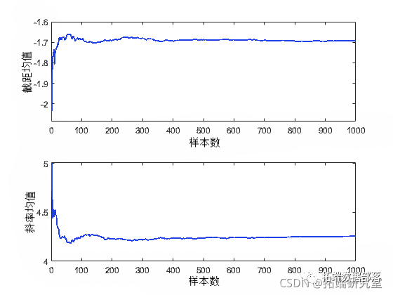
In this case, a sample size of 1000 seems sufficient to provide good accuracy for the posterior mean estimates.
mean(te)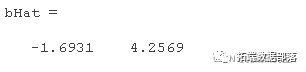
Summary
You can easily specify the likelihood and prior. You can also combine them for inferring the posterior distribution. You can perform Bayesian analysis in MATLAB using Markov Chain Monte Carlo simulations.

The data and code analyzed in this article are shared in the member group. Scan the QR code below to join the group!


Click “Read the original” at the end of the article to obtain the complete data
This article is excerpted from “Analysis of Automotive Experimental Data Using Logistic Regression Model with Markov Chain Monte Carlo (MCMC) in MATLAB”.

Click the title to check previous content
R language coda Bayesian MCMC Metropolis-Hastings sampling chain analysis and convergence diagnostic visualizationR language implementation of the Metropolis–Hastings algorithm and Gibbs sampling in MCMCR language Bayesian METROPOLIS-HASTINGS GIBBS Gibbs sampler estimation of change point exponential distribution analysis of Poisson process station waiting timeR language Markov MCMC METROPOLIS HASTINGS, MH algorithm sampling (sampling) visualization examplePython Bayesian stochastic processes: Markov chain Markov-Chain, MC and Metropolis-Hastings, MH sampling algorithm visualizationPython Bayesian inference Metropolis-Hastings (M-H) MCMC sampling algorithm implementationMetropolis Hastings sampling and Bayesian Poisson regression Poisson modelMatlab using BUGS Markov switching random volatility model, sequential Monte Carlo SMC, M H sampling analysis of time seriesR language RSTAN MCMC: NUTS sampling algorithm using LASSO to build Bayesian linear regression model analysis of occupational prestige dataR language BUGS sequential Monte Carlo SMC, Markov switching random volatility SV model, particle filtering, Metropolis Hasting sampling time series analysisR language Metropolis Hastings sampling and Bayesian Poisson regression Poisson modelR language Bayesian MCMC: using rstan to build linear regression model analysis of automotive data and visualization diagnosticsR language Bayesian MCMC: GLM logistic regression, Rstan linear regression, Metropolis Hastings and Gibbs sampling algorithm examplesR language Bayesian Poisson normal distribution model analysis of occupational football match goalsR language using Rcpp to accelerate Metropolis-Hastings sampling to estimate Bayesian logistic regression model parametersR language logistic regression, Naive Bayes, decision tree, random forest algorithms predicting heart diseaseR language Bayesian networks (BN), dynamic Bayesian networks, linear model analysis of malocclusion dataR language block Gibbs sampling Bayesian multivariate linear regressionPython Bayesian regression analysis of housing affordability datasetR language implementation of Bayesian quantile regression, lasso and adaptive lasso Bayesian quantile regression analysisPython implementing Bayesian linear regression model with PyMC3R language using WinBUGS software to establish hierarchical (layered) Bayesian models for academic ability testsR language Gibbs sampling Bayesian simple linear regression simulation analysisR language and STAN, JAGS: using RSTAN, RJAG to establish Bayesian multivariate linear regression to predict election dataR language based on copula Bayesian hierarchical mixture model diagnostic accuracy studyR language Bayesian linear regression and multivariate linear regression to build salary prediction modelsR language Bayesian inference and MCMC: implementation of Metropolis-Hastings sampling algorithm exampleR language stan for regression models based on Bayesian inferenceR language RStan Bayesian hierarchical model analysis exampleR language using Metropolis-Hastings sampling algorithm adaptive Bayesian estimation and visualizationR language random search variable selection SSVS estimation of Bayesian vector autoregression (BVAR) modelWinBUGS for multivariate random volatility model: Bayesian estimation and model comparisonR language implementation of Metropolis–Hastings algorithm and Gibbs sampling in MCMCR language Bayesian inference and MCMC: implementation of Metropolis-Hastings sampling algorithm exampleR language using Metropolis-Hastings sampling algorithm adaptive Bayesian estimation and visualizationVideo: Bayesian models of Stan probability programming MCMC sampling in R languageR language MCMC: Metropolis-Hastings sampling for Bayesian estimation in regressionR language logistic regression, Naive Bayes, decision tree, random forest algorithms predicting heart diseaseR language logistic regression (Logistic Regression), regression decision tree, random forest credit card default analysis credit data setPYTHON user churn data mining: building logistic regression, XGBOOST, random forest, decision tree, support vector machine, naive Bayes and KMEANS clustering user portraitsPython modeling and forecasting sales time series analysis of store data using LSTM and XGBOOSTPYTHON ensemble machine learning: using ADABOOST, decision tree, logistic regression ensemble model classification and regression and grid search hyperparameter optimizationR language ensemble models: boosting trees, random forests, constrained least squares weighted average model fusion analysis of time series dataPython modeling and forecasting sales time series analysis of store data using LSTM and XGBOOSTR language using principal component PCA, logistic regression, decision tree, random forest to analyze heart disease data and high-dimensional visualizationR language tree-based methods: decision trees, random forests, Bagging, boosting treesR language classification prediction of credit data set using logistic regression, decision tree and random forestSPSS modeler using decision tree neural networks to predict ST stocksR language using linear models, regression decision trees to automatically combine feature factor levelsR language implementing CART regression decision trees with self-defined Gini coefficientR language using rle, svm and rpart decision trees for time series forecastingPython predicting NBA winners using decision trees and random forests in Scikit-learnPython classification modeling and cross-validation of iris flower data using decision trees in scikit-learn and pandasNonlinear models in R language: polynomial regression, local splines, smooth splines, generalized additive models GAM analysisR language using standard least squares OLS, generalized additive models GAM, spline functions for logistic regression LOGISTIC classificationR language ISLR wage data for polynomial regression and spline regression analysisPolynomial regression, local regression, kernel smoothing and smooth spline regression models in R languageR language using Poisson regression, GAM spline curve models to predict the number of cyclistsR language quantile regression, GAM spline curves, exponential smoothing and SARIMA for power load time series forecastingR language spline curves, decision trees, Adaboost, gradient boosting (GBM) algorithms for regression, classification and dynamic visualizationHow to build ensemble models in machine learning using R language?R language ARMA-EGARCH model, ensemble forecasting algorithms for predicting SPX actual volatilityCalculating neural network ensemble models in deep learning Keras in PythonR language ARIMA ensemble model for time series analysisR language based on Bagging classification of logistic regression (Logistic Regression), decision trees, forests to analyze heart disease patientsR language tree-based methods: decision trees, random forests, Bagging, boosting treesR language based on Bootstrap linear regression prediction confidence interval estimation methodR language using bootstrap and incremental methods to calculate generalized linear model (GLM) prediction confidence intervalsR language spline curves, decision trees, Adaboost, gradient boosting (GBM) algorithms for regression, classification and dynamic visualizationPython modeling and forecasting sales time series analysis of store data using LSTM and XGBOOSTR language random forest RandomForest, logistic regression Logistic prediction of heart disease data and visualization analysisR language using principal component PCA, logistic regression, decision tree, random forest to analyze heart disease data and high-dimensional visualizationMatlab establishing SVM, KNN and naive Bayes model classification drawing ROC curvesMatlab using quantile random forest (QRF) regression trees to detect outliers