Note: This is a practical machine learning project (including data + code + documentation), if you need data + code + documentation you can directly obtain it at the end of the article.

1. Project Background

Breast cancer is one of the most common cancers among women worldwide, and early diagnosis is crucial for improving cure rates and survival rates. Traditional diagnostic methods rely on the experience of doctors and pathological analysis, which are not only time-consuming but also susceptible to subjective factors. With the development of machine learning technologies, it has become possible to automatically classify and predict medical images and data using algorithms such as Support Vector Machines (SVM). This project aims to develop an efficient and accurate breast cancer classification method based on the MATLAB platform, by applying the SVM algorithm to train and test breast cancer-related datasets, achieving effective identification and classification of breast cancer. This system can not only assist doctors in making faster and more accurate diagnoses but also provide a reference for personalized treatment plans, thereby improving medical efficiency and patient satisfaction. Additionally, this project will explore the impact of different feature selection methods on model performance, with the goal of finding the optimal breast cancer classification strategy.

This project implements the application of SVM support vector machine for breast cancer classification based on MATLAB.

2. Data Acquisition

The modeling data is sourced from the internet (compiled by the author of this project), and the data items are summarized as follows:

No.	Variable Name	Description
1	radius1	Mean radius
2	texture1	Mean texture
3	perimeter1	Mean perimeter
4	area1	Mean area
5	smoothness1	Mean smoothness
6	compactness1	Mean compactness
7	concavity1	Mean concavity
8	concave_points1	Mean number of concave points
9	symmetry1	Mean symmetry
10	fractal_dimension1	Mean fractal dimension
11	radius2	Standard error of radius
12	texture2	Standard error of texture
13	perimeter2	Standard error of perimeter
14	area2	Standard error of area
15	smoothness2	Standard error of smoothness
16	compactness2	Standard error of compactness
17	concavity2	Standard error of concavity
18	concave_points2	Standard error of number of concave points
19	symmetry2	Standard error of symmetry
20	fractal_dimension2	Standard error of fractal dimension
21	radius3	Mean of the maximum three radius values
22	texture3	Mean of the maximum three texture values
23	perimeter3	Mean of the maximum three perimeter values
24	area3	Mean of the maximum three area values
25	smoothness3	Mean of the maximum three smoothness values
26	compactness3	Mean of the maximum three compactness values
27	concavity3	Mean of the maximum three concavity values
28	concave_points3	Mean of the maximum three number of concave points
29	symmetry3	Mean of the maximum three symmetry values
30	fractal_dimension3	Mean of the maximum three fractal dimension values
31	y	Whether the tumor is benign (0) or malignant (1)

Data details are as follows (partial display):

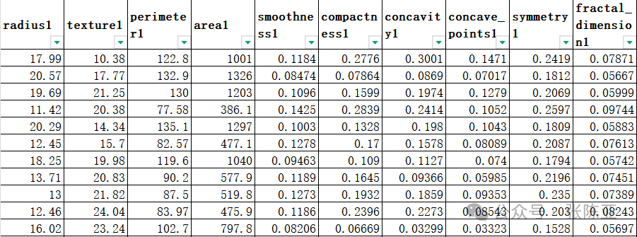
3. Data Preprocessing

3.1 View Data

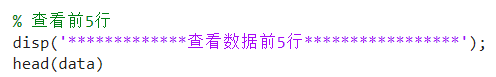
Use the head() method to view the first five rows of data:

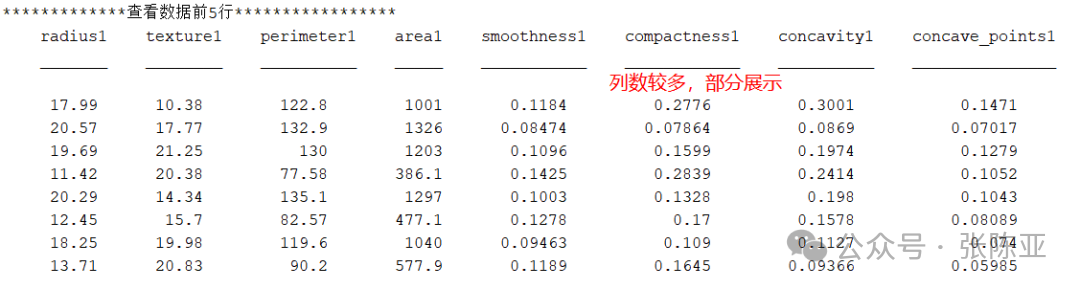
Key code:

3.2 Check for Missing Data and Descriptive Statistics

Use the summary() method to view data information:

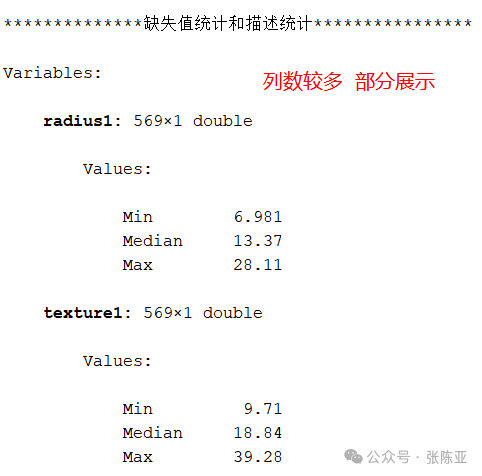
From the above figure, it can be seen that there are a total of 31 variables, with no missing values in the data, totaling 569 data entries.

Key code:

4. Exploratory Data Analysis

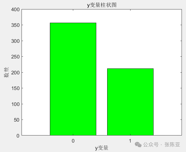
4.1 Bar Chart of Independent Variables

Use the bar() method to draw a bar chart:

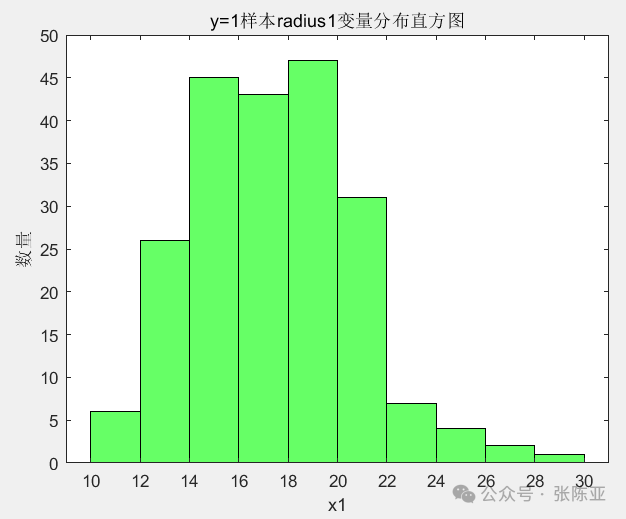
4.2 Histogram of radius1 Variable for y=1 Samples

Use the histogram() method to draw a histogram:

4.3 Correlation Analysis

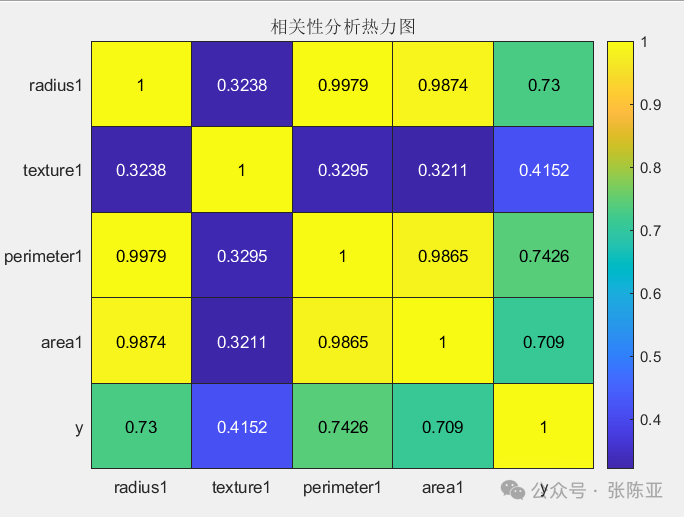
Correlation analysis of some data variables: From the above figure, it can be seen that the larger the value, the stronger the correlation; positive values indicate positive correlation, while negative values indicate negative correlation.

5. Feature Engineering

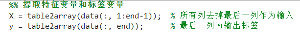
5.1 Establish Feature Data and Label Data

Key code is as follows:

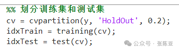
5.2 Dataset Splitting

Split into 80% training set and 20% validation set, key code is as follows:

6. Build SVM Classification Model

Mainly implements the application of SVM support vector machine for breast cancer classification based on MATLAB..

6.1 Build Model

Build classification model.

Model Name	Model Parameters
SVM Classification Model	‘KernelFunction’, ‘linear’
‘Standardize’, true
‘ClassNames’, [0, 1]

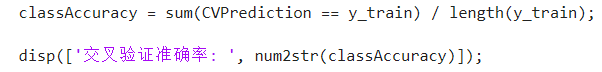
6.2 Cross-Validation to Optimize Parameters

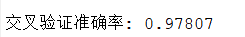
Key code:

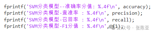
7. Model Evaluation

7.1 Evaluation Metrics and Results

Evaluation metrics mainly include accuracy, precision, recall, F1 score, etc.

Model Name	Metric Name	Metric Value
Test Set
SVM Classification Model	Accuracy	0.9735
Precision	1.0000
Recall	0.9286
F1 Score	0.9630

From the above table, it can be seen that the F1 score is 0.9630, indicating that the model performs well..

Key code is as follows:

7.2 Confusion Matrix

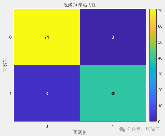
From the above figure, it can be seen that there are 0 samples predicted as not 0 when the actual value is 0, and 3 samples predicted as not 1 when the actual value is 1, indicating that the model performs well..

8. Conclusion and Outlook

In summary, this project implements the application of SVM support vector machine for breast cancer classification based on MATLAB, ultimately proving that the model we proposed performs well. This model can be used for daily product modeling work.

Project practical collection navigation:

https://docs.qq.com/sheet/DTVd0Y2NNQUlWcmd6?tab=BB08J2           

Python Project Collection

Graduation Project System

MATLAB Project Collection

Special Training Camp

Thesis Full Package, Half Package Services

Data Collection

Free Material Acquisition

R Project Collection

——Welcome to follow our public account——