GNSS_AOA filtering, using the concept of tight coupling between GNSS and AOA for the fusion filtering of three sensors, EKF, in a two-dimensional environment. The fused data includes: GNSS XY position, AOA angle information, and speed information collected from inertial navigation or dead reckoning.

Table of Contents

• Program Overview
• 1. System Overview
• 2. Function Overview
• 3. Main Steps
• 4. Performance Comparison
• Running Results
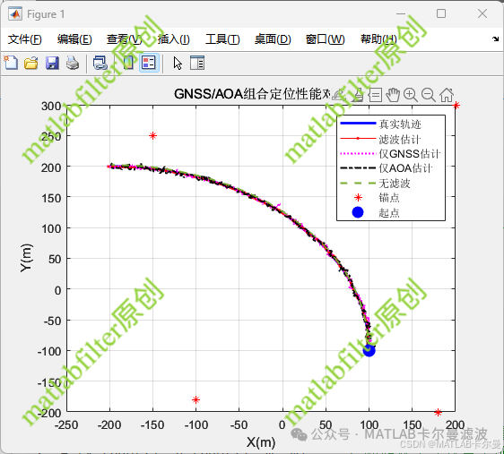
• Positioning Diagram (Trajectory Comparison)
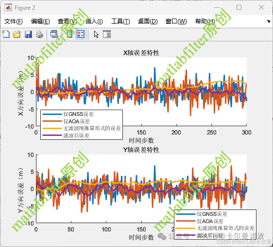
• Error Curve
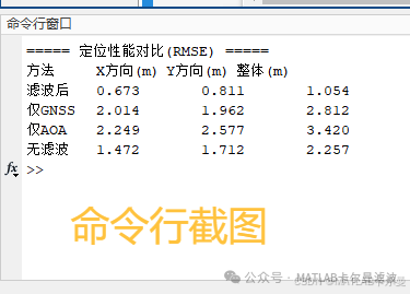
• Error Characteristics from Command Line Output
• MATLAB Code
• Program Structure
• Partial Code
• Complete Code

Program Overview

This code implements a tight coupling positioning algorithm based on GNSS (Global Navigation Satellite System) and AOA (Angle of Arrival) information, primarily using Extended Kalman Filtering (EKF) for multi-sensor data fusion to estimate the position and speed of objects in a two-dimensional environment. The code demonstrates the positioning performance of GNSS and AOA data fusion through simulated trajectories, measurement data, and filtered estimation results.

1. System Overview

The system combines observation data from three main sensors:

• GNSS provides geographical location information of the object (longitude and latitude).
• AOA (Angle of Arrival) provides the angular relationship between the object and multiple anchor points.
• Speed Information, typically sourced from an Inertial Measurement Unit (IMU) or gait estimation.

These sensor data are fused using a Kalman filter to improve positioning accuracy and system robustness.

2. Function Overview

• Initialize Parameters: Set time step, total duration, random noise parameters, etc.
• Trajectory Generation: Generate the actual object motion trajectory based on predetermined angle changes and radius.
• Simulated Measurement: Generate simulated data for GNSS, AOA, and speed information by adding random noise.
• Extended Kalman Filtering (EKF): Continuously fuse observation data from different sensors through prediction and update steps to optimize the object’s positioning estimate.
• Performance Evaluation: Evaluate the positioning accuracy of different data fusion schemes (e.g., GNSS, AOA, filtered estimates) through error analysis and comparison.

3. Main Steps

1. Initialization: Set state variables (position and speed), process noise, and measurement noise.

2. Data Generation:

• The true trajectory is generated using predetermined mathematical formulas (based on angle and radius).
• GNSS measurement data is generated by adding noise to the true position.
• AOA data is generated by simulating the angular relationship between satellites and the target.

Filtering Process:

• Predict the next state using the state transition function.
• Update the prediction results using the Kalman gain, fusing GNSS and AOA measurements.
• After each update, the state and covariance matrix are updated.

Result Presentation:

• Visualize the trajectory comparisons of different estimation methods (GNSS only, AOA only, filtered, unfiltered).
• Statistical errors, including RMSE (Root Mean Square Error) and other evaluation metrics.
• Unidirectional error analysis, showing positioning errors for the X-axis and Y-axis separately.

4. Performance Comparison

The code demonstrates the error performance of different algorithms in positioning through various trajectory comparisons:

• Filtered Estimate: Achieved relatively accurate positioning by fusing GNSS and AOA information through EKF.
• GNSS Only Estimate: Positioning using only GNSS data, typically resulting in larger errors.
• AOA Only Estimate: Positioning using only AOA data, with errors depending on the layout of anchor points and angle accuracy.
• No Filtering Estimate: Updating estimated position through pure estimation (no filtering), usually resulting in larger and unstable errors.

Running Results

Positioning Diagram (Trajectory Comparison)

Error Curve

Error Characteristics from Command Line Output

MATLAB Code

Program Structure

Partial Code

% GNSS_AOA filtering, using the concept of tight coupling between GNSS and AOA for the fusion filtering of three sensors, EKF, in a two-dimensional environment
% The fused data includes: GNSS XY position, AOA angle information, and speed information collected from inertial navigation or dead reckoning
% Author WeChat: matlabfilter, can customize programs related to positioning and navigation

clc; clear; close all;
rng(0);% Fix random seed to ensure consistent results

%% Initialize Parameters
dt =1;% Time step (s)
T =300;% Total duration
N = T/dt;% Number of time steps

% Generate true trajectory
theta =linspace(0,pi/2, N);% Generate an angle sequence from 0 to π/2
radius =300;% Radius
x_true = radius *cos(theta)-200;% Calculate true X coordinate
y_true = radius *sin(theta)-100;% Calculate true Y coordinate

% Calculate true trajectory speed information
vel_true =[
0,diff(x_true);% Change in speed on X-axis
0,diff(y_true)]/ dt;% Change in speed on Y-axis

% Initial state variables [x, y, vx, vy]
X_est =[x_true(1);y_true(1);0;0];% Initial estimated state (position and speed)
X_ =[x_true(1);y_true(1);0;0];% Initial state (used only for prediction)
P =diag([10,10,1,1]);% Initial covariance matrix, assuming large uncertainty in position and small in speed

% Process noise parameters
Q =0.1*diag([0.1,0.1,0.05,0.05]);% Define process noise covariance

% Anchor point parameters (simulating 4 satellites)
anchor_pos =[
200300;
-150250;
180-200;
-100-180];% Define positions of four satellites
num_sats =size(anchor_pos,1);% Calculate number of satellites

% Observation noise parameters
R_gnss =2^2*diag([1,1]);% GNSS position measurement noise
R_aoa =0.01^2*eye(4);% AOA angle measurement noise

%% Generate simulated measurement data
[meas_aoa]=generate_measurements(x_true, y_true, anchor_pos, R_aoa);% Generate AOA measurement data
meas_GNSS =[x_true; y_true]+sqrt(diag(R_gnss)).*randn(2, N);% Add GNSS measurement noise

traj_gnss =zeros(2, N);% Store only GNSS trajectory
traj_aoa =zeros(2, N);% Store only AOA trajectory
traj_est =zeros(4, N);% Store filtered trajectory (including position and speed)
X_s =zeros(4, N);% Store purely estimated trajectory

Complete Code Download Link:

https://mall.bilibili.com/neul-next/detailuniversal/detail.html?isMerchant=1&page=detailuniversal_detail&saleType=10&itemsId=12642349&loadingShow=1&noTitleBar=1&msource=merchant_share

Or click on “Read the original text” at the end to jump.

<span>If you need assistance or have customization requirements for navigation and positioning filtering codes, please contact the author via WeChat below</span>