💥💥💞💞Welcome to this blog❤️❤️💥💥
🏆Author’s Advantage: 🌞🌞🌞The blog content aims to be logically clear and coherent for the convenience of readers.
⛳️Motto: A journey of a hundred miles begins with a single step.
💥1 Overview
1.1 Dynamic Analysis of Electrical Systems
This task mainly involves a deep study of the concepts learned in class, highlighting one of the most significant aspects of embedded systems: the large-scale use of power electronic converters.
The application will be based on very simple examples, allowing for a comparison of time simulation results with analytical calculations learned in class. The simulation software may use PSIM, as it is user-friendly and performs excellently.
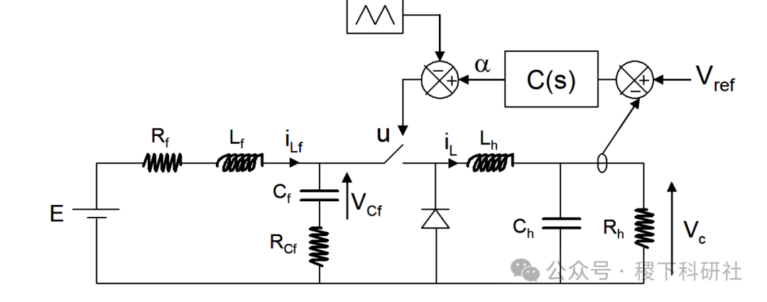
This dynamic study will involve the case of a series chopper with an input filter discussed in the course, structured as shown below. Parameters for this chopper will also be provided.
Chopper Characteristics
E = 350 V DC Power = 5 kW Vc = 28 V DC
Lh = 290 H Ch = 400 F fh = 5 kHz

Filter
Rf = 250 m Lf = 200 H Cf = 100 F RCf = 0
Preparation:
– Consider that only the output voltage Vc is adjusted by changing the triggering angle α of the chopper, and determine the open-loop and closed-loop state-space models of the system.
– Determine the maximum frequency of the effective domain of the average model based on the system parameters.
– Define two dynamic performance requirements for the system (response time, overshoot, stability margin, etc.):
Can be regulation
Can also be tracking
(1) Analysis Study: Modal Method of Stability
Based on the open-loop state-space model, calculate the participation factors and sensitivity, and conduct a complete stability analysis of the system.
Particular attention should be paid to the most critical parameters in the system, and analyze the movement of the system poles after a 100% change in these parameters relative to their nominal values.
(2) System Control
Using Matlab’s Sisotool, design two controllers:
ü Either with good performance (response time, damping);
ü Or with good robustness (gain and phase margin).
Analyze the frequency response of the sensitivity function S using these two controllers.
(3) Simulation: Verification
Perform closed-loop simulation of the system using the “validation_BF.sch” file (PSIM simulation).
Evaluate the performance of the controller when the load disturbance is 5% or 50%. Analyze the robustness of the controller when parameters change significantly (especially the critical parameters from part 2).
(4) Summarize the design of the system
1.2 Urban Rail Transit Power Supply System
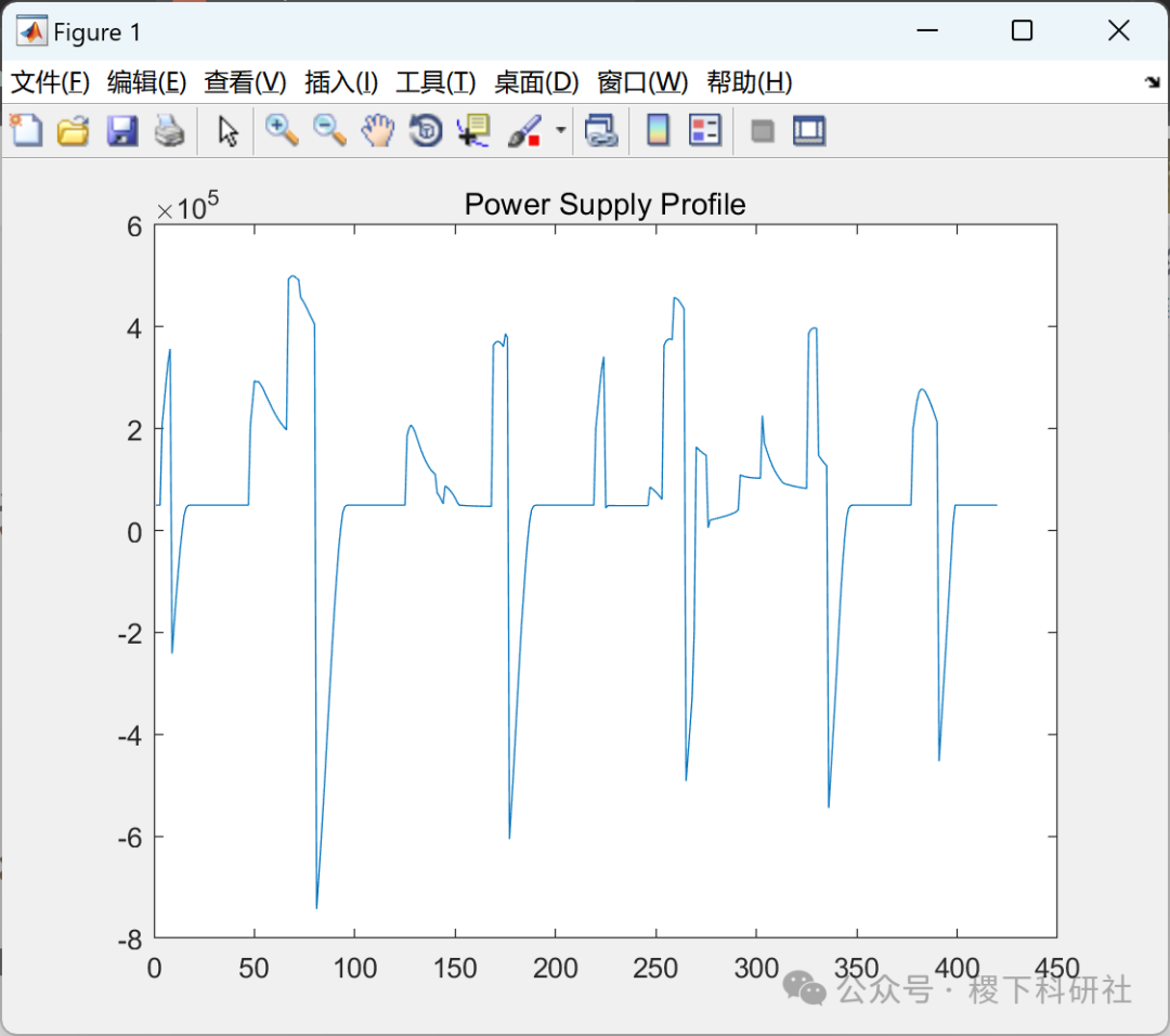
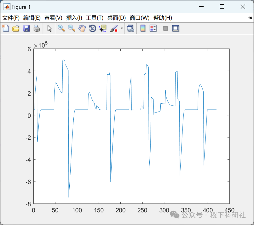
Consider moving a CITADIS type tram on a test line of up to 1.5 kilometers. The power (Pelec) of the vehicle on the contact wire is shown in Figure 1.
The sampling profile with a sampling period of 1 second is described in the file donnees.mat. Calculations can be performed in the Matlab© environment.
1) Characterization of Load Profile
Based on the power profile to be provided, determine the Power Hybrid Potential (PHP) and Energy Hybrid Potential (PHE). Conclusions will be drawn regarding the selection of hybrid drive systems and auxiliary sources (energy storage).
We then choose the following symbol conventions:
-
In traction mode, Pelec is positive (corresponding to the discharge phase of energy storage);
-
In braking mode, Pelec is negative (corresponding to the charging phase of energy storage).
2) Energy Storage Technology Selection
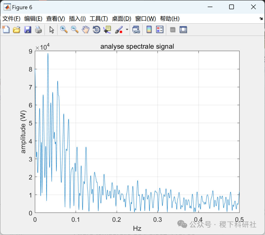
Using the spectre.m function, determine the spectrum of the load profile. Conclusions will be drawn regarding the selected energy storage technology.
Next, we assume that the average power of the profile will be provided by the EDF network connected to the tram system under study. The remaining required power will be provided by the considered energy storage.
Select to address either problem 3) or 4). Finally, there is a common problem 5).
3) Supercapacitor Energy Storage
3.a) Calculations:
-
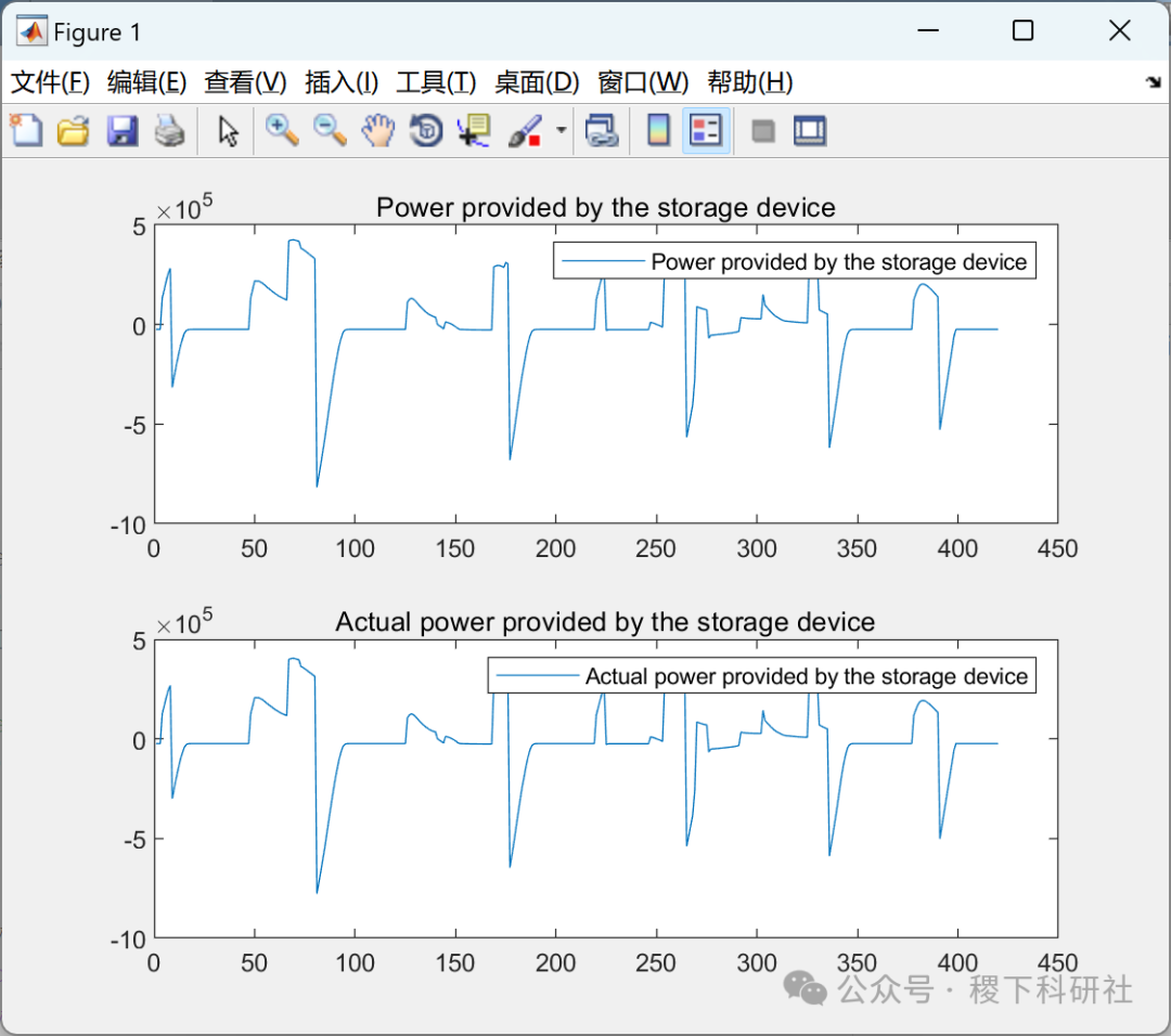
Energy storage power calculated at the energy connection node;
-
Actual power converted to energy storage, assuming the overall conversion efficiency of the supercapacitor (losses in the converter and storage medium) is 95%;
-
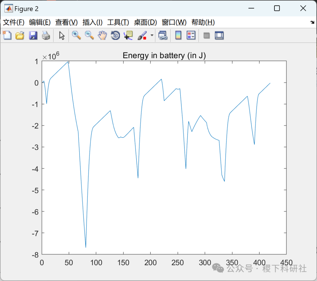
Energy actually stored in the supercapacitor.
3.b) Derive (ignoring losses in the capacitor combination):
-
Energy storage required to perform the task;
-
Total capacity of the capacitor combination (average depth of discharge 75%);
-
Maximum power charged or discharged in the supercapacitor combination;
-
Energy storage power calculated at the energy connection node;
-
Actual power converted to energy storage, assuming the overall conversion efficiency of the battery (losses in the converter and storage medium) is 81%;
-
Energy actually stored in the battery;
-
Considering the saturation of the charging state, energy storage in the battery pack. For this, we will set the energy at the start of the task to zero. The actual stored energy can be compared with the energy calculated through saturation integration.
-
Energy storage required to perform the task;
-
Total capacity of the battery pack (average depth of discharge 50%);
-
Maximum power charged and discharged in the battery pack;
-
Based on the technical elements given in Table 2, size the battery pack (number of elements, recommended voltage and current, volume, and total volume). Observed characteristics can be marked on the capacity/discharge power plane. We will not attempt to optimize the sizing of the selected battery.
4) High Power Density Battery Case
4.a) Calculations:
4.b) Derive:
5) Study the sensitivity of sizing design to the power provided by the EDF network. This can be studied by modifying the set values by ±50% each time.
1.3 Analysis of Operating Results
This section is a detailed analysis of the test results, see section 4.


📚2 Operating Results
2.1 Test 1


2.2 Test 2


2.3 Test 3



Partial Code:
close all
clc
clear
load Tram.mat
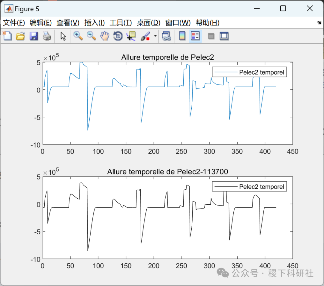
Pelec2=zeros(size(T,2),1);
for i=1:size(T,2)
Pelec2(i,1)=T(1,i).pelec;
end
% Calculating the mean of the energy demand
Pmoy=mean(Pelec2)
figure
subplot(2,1,1)
plot (Pelec2-Pmoy)
legend(‘Power provided by the storage device’);
title(‘Power provided by the storage device’);
ActualPelec2=zeros(size(Pelec2,1),1);
for i=1:size(Pelec2,1)
if(Pelec2-Pmoy)>0
ActualPelec2(i,1)=(Pelec2(i,1)-Pmoy)/0.95;
else
ActualPelec2(i,1)=(Pelec2(i,1)-Pmoy)*0.95;
end
end
subplot(2,1,2)
plot(ActualPelec2)
legend(‘Actual power provided by the storage device’);
title(‘Actual power provided by the storage device’);
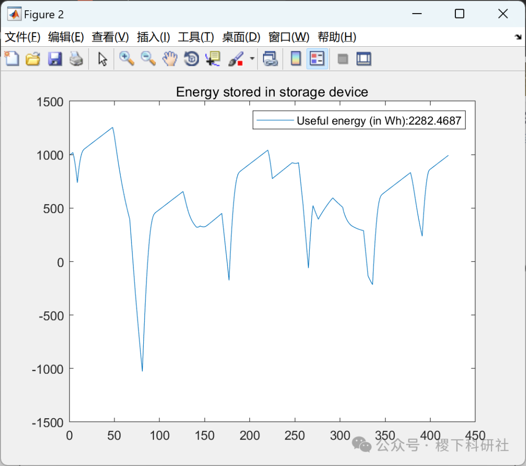
energyStoredInWh=zeros(size(ActualPelec2,1),1);
energyStoredInWh(1,1)=1000;
for i=2:size(ActualPelec2,1)
energyStoredInWh(i,1)=energyStoredInWh(i-1,1)-(ActualPelec2(i-1,1)/(60*60));
end
figure;
plot(energyStoredInWh)
legend(strcat(‘Useful energy (in Wh): ‘,num2str(max(energyStoredInWh)-min(energyStoredInWh))));
title(‘Energy stored in storage device’);
disp(strcat(‘Useful energy: ‘,num2str(max(energyStoredInWh)-min(energyStoredInWh))));
% Assuming 75 percent DoD, the capacity energy capacity can be calculated
capEnergyCapacityInWh=(max(energyStoredInWh)-min(energyStoredInWh))*4/3
% The maximum power imposed upon the capacitor can also be calculated
maxPowerImposedInW=max(ActualPelec2)
voltageInV=2.5;
capacitorInF=5000;
esrInuOhms=350;
% The total capacitance of the package can be calculated using the capacity energy
% energy capacity
totalCapacityInF=2capEnergyCapacityInWh60*60/((voltageInV)^2);
disp(strcat(‘Total capacity required in farads assuming voltage of one capacitor: ‘, num2str(totalCapacityInF)));
% voltageInV=2.5;
% capacitorInF=5000;
% esrInuOhms=350;
% the energy capacity of one pack
energyInOnePackInWh=capacitorInF(voltageInV^2)/(26060)maximalPowerInOneElementInW=0.12(voltageInV^2)/(esrInuOhms/1000000)
% Number of capacitors required according to energy capacity and power
% capacity
NumOfCapEnergy=capEnergyCapacityInWh/energyInOnePackInWh
NumOfCapPower=maxPowerImposedInW/maximalPowerInOneElementInW
disp(strcat(‘Number of capacitors required: ‘, num2str(ceil(max(NumOfCapEnergy,NumOfCapPower)))))
🎉3 References
Some content in this article is sourced from the internet, and references will be noted or cited as references. If there are any inaccuracies, please feel free to contact for removal.
[1] Li Jianmin, Sun Jianshe. Research on Harmonic Distribution of Urban Rail Transit Power Supply System [J]. Electric Measurement and Instrumentation, 2008, 45(2):6. DOI:10.3969/j.issn.1001-1390.2008.02.001.
[2] Chen Runzhi. Research on the Design of Urban Rail Transit Power Supply System [J]. Electronic Magazine of Encyclopedia Forum, 2019, 000(004):471.
[3] Wang Guoliang. Research on a Certain Urban Rail Transit Power Supply System [D]. North China Electric Power University [2023-12-31]. DOI:CNKI:CDMD:2.1016.276128.
🌈4 Matlab Code, Data, Document Explanation