

Click the blue text above to follow us


Gift to readers
👨💻 Conducting research involves a profound system of thought, requiring researchers to be logical, meticulous, and serious. However, effort alone is not enough; often leveraging resources is more important than hard work. Additionally, one must have innovative and inspirational points of view. When a philosophy teacher asks you what science is or what electricity is, do not find these questions amusing. Philosophy is the mother of science; it seeks to address ultimate questions and find those self-evident questions that only children would ask but you cannot answer. Readers are advised to browse through the content in order to avoid suddenly falling into a dark maze without finding their way back. This article may not reveal all the answers to your questions, but if it can spark clouds of doubt in your mind, it may create a beautiful sunset of thoughts. If it brings you a storm in your spiritual world, then take the opportunity to brush off the dust that has settled on your ‘lying flat’ mindset.
Perhaps, after the rain, the sky will be clearer…….🔎🔎🔎

1 Overview
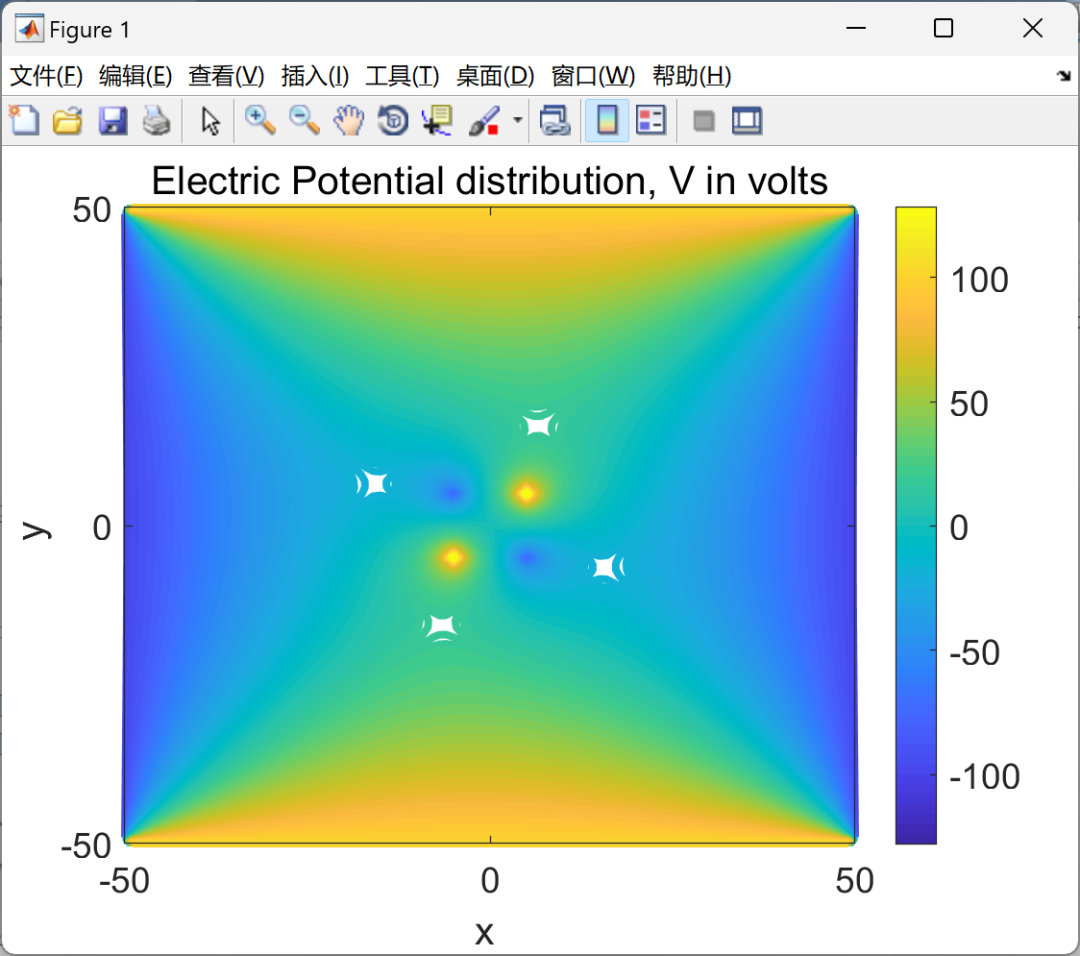
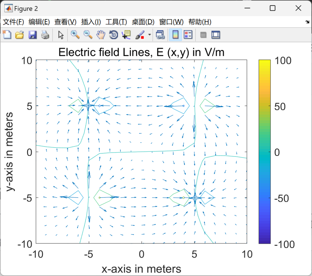
This paper calculates the electric field generated by a pair of dipoles by solving Poisson’s equation using the finite difference method to compute the electric field produced by two dipoles in a two-dimensional plane. In this study, the boundary conditions for Poisson’s equation are defined by alternating known potentials of 100V and -100V on the four boundary walls. Two identical dipoles with charges of 2nC are placed at x=10 and x=-10. Poisson’s equation is iteratively solved using the finite difference method (FDM).The solution to Poisson’s equation is plotted as equipotential contours. The electric field is calculated using the gradient function and is also displayed as an arrow diagram.
This research focuses on solving complex physical problems through numerical methods, specifically targeting the calculation of the fine electric field distribution generated by a pair of dipoles in two-dimensional space. The core technique we employ is the classical finite difference method (FDM) to solve Poisson’s equation, which describes the potential distribution. This method not only reflects a clever combination of theory and practice but also showcases the powerful capabilities of mathematical tools in analyzing natural phenomena.
The article elaborates on how to utilize the FDM framework to accurately simulate the influence of a dipole system composed of two equal but opposite charges (each dipole having a charge of 2nC) on the surrounding electric field in a clearly defined two-dimensional plane. These two dipoles are symmetrically positioned at ±10 on the x-axis, designed to create a typical and easily analyzable electric field model.
To accurately simulate real-world conditions, we impose non-trivial boundary conditions on the four boundaries of the system: the potential is maintained at 100V and -100V on opposite walls, creating a dynamic and challenging potential distribution environment. This approach effectively simulates the complex electric field constraints that may be encountered in reality, enhancing the practical value and applicability of the research.
Through a carefully designed algorithm executing multiple iterations, we successfully obtained the precise solution to Poisson’s equation. To visually demonstrate the spatial distribution characteristics of the potential, the results are artistically transformed into a series of equipotential contour plots. These contours not only clearly outline the trend of potential variation with space but also provide visual support for a deeper understanding of the characteristics of the electric field under the interaction of the dipoles.
Furthermore, this paper derives the distribution of electric field strength directly from the solution by calculating the gradient of the potential and presents it in the form of an arrow diagram. This intuitive representation not only reveals the directionality of the electric field but also accurately depicts the variation in electric field strength, providing readers with a comprehensive and profound understanding perspective.
In summary, this study innovatively applies the finite difference method to solve Poisson’s equation, successfully simulating the distribution characteristics of the electric field of dipoles, and has made significant strides in visual expression and deepening the understanding of physical concepts, providing valuable references and insights for research in related fields.
2Results
% Part of the code:Q = [2,-2,-2,2]*charge_order; % What are the charges?% Array of charge locations (Actual coordinates in a Cartesian Plane)X = 0.5*[10,10,-10,-10]; % Where are the charges located?Y = 0.5*[10,-10,10,-10];X = X + mpx; % Relative coordinates for computationY = Y + mpy;Rho = zeros(Nx,Ny); % Charge distribution matrixfor k = 1:n % Loop through all chargesRho(X(k),Y(k)) = Q(k)/eps;end%-------------------------------------------------------------------------% Computing potentials in the box%-------------------------------------------------------------------------%for l = 1:n % Repeat for all chargesfor z = 1:Ni % Number of iterations
3References
Some content in this article is sourced from the internet, and references will be noted or cited as references. If there are any inaccuracies, please feel free to contact us for removal.

[1] Hu Xianquan, Xu Jie, Ma Yong, et al. Study on Charge Confinement of Electric Dipoles [J]. Journal of Yunnan University: Natural Science Edition, 2005, 27(S2):61-66. DOI: CNKI:SUN:YNDZ.0.2005-S2-011.
[2] Geng Xueying, Zhang Qilin, Liu Mingyuan. Simulation Study on the Impact of Ground Buildings on Thunderstorm Cloud Atmospheric Electric Field [C]// 28th Annual Meeting of the Chinese Meteorological Society. 0 [2024-07-07].
[3] Hui Zhejian. Research on Time-Domain Marine Electromagnetic Three-Dimensional Forward and Inverse Problems Based on Unstructured Finite Element Method [D]. Jilin University [2024-07-07].
4 MATLAB Code Implementation
For more resources and benefits for fans, MATLAB | Simulink | Python resources available