Research on Optimal Scheduling Scheme for Pumped Storage Power Station Based on MATLAB Particle Swarm AlgorithmReferences: Research on Optimal Scheduling Scheme for Pumped Storage Power Station Non-Complete ReproductionMATLAB + Particle Swarm AlgorithmMain Content: This study investigates the peak shaving and valley filling functions of pumped storage units, aiming to minimize costs while considering the interests of the power grid, the operational environment of the pumped storage power station, and the existing peak shaving pricing mechanisms of various power sources, to develop an economic scheduling model for a mixed power generation system that includes pumped storage units. Then, the particle swarm algorithm is combined with the economic scheduling model of the mixed power generation system containing pumped storage units to derive specific steps for solving the system’s day-ahead scheduling problem.

The following text and example code are for reference only

Table of Contents

• Research on Optimal Scheduling Scheme for Pumped Storage Power Station Based on MATLAB Particle Swarm Algorithm
• Project Overview
• Problem Description
• MATLAB Code Implementation
• System Description and Analysis
• 1. Algorithm Flow
• 2. Cost Function Design
• 3. Water Level Dynamic Model
• 4. Optimization Results
• Parameter Tuning Suggestions
• Improvement Directions

Research on Optimal Scheduling Scheme for Pumped Storage Power Station Based on MATLAB Particle Swarm Algorithm

Project Overview

This project utilizes the Particle Swarm Optimization (PSO) algorithm to solve the optimal scheduling scheme for pumped storage power stations. The goal is to minimize generation costs and maximize energy efficiency while meeting the power system demand and operational constraints of the power station.

Problem Description

Pumped storage power stations play a crucial role in the power system, allowing water to be pumped for energy storage during low demand periods and generating power during peak demand. Our problem is to determine the optimal scheduling scheme that:

• Meets power demand
• Minimizes operational costs
• Maximizes energy conversion efficiency
• Adheres to equipment operational constraints

MATLAB Code Implementation

% Particle Swarm Optimization Algorithm for Pumped Storage Power Station Scheduling Optimization

% Clear workspace
clear;
clc;
close all;

%% Parameter Settings
numParticles = 50; % Number of particles
numVariables = 24; % Number of decision variables (one decision per hour)
maxIterations = 100; % Maximum number of iterations
w = 0.729; % Inertia weight
c1 = 1.494; % Individual learning factor
c2 = 1.494; % Social learning factor

% Operational constraints
minPower = zeros(1, numVariables); % Minimum output
maxPower = 300 * ones(1, numVariables); % Maximum output (MW)
minWaterLevel = 50; % Minimum water level (%)
maxWaterLevel = 90; % Maximum water level (%)
initialWaterLevel = 80; % Initial water level

% Load demand (example: 24-hour load forecast)
loadDemand = [5050607080100120150...
180200220250...
220200180150...
120100807060505050];

%% Initialize Particle Swarm
particles = rand(numParticles, numVariables) .* repmat(maxPower, numParticles, 1);
velocities = rand(numParticles, numVariables);

% Calculate initial fitness
pbest = particles;
pbestCost = zeros(numParticles, 1);
for i = 1:numParticles
    pbestCost(i) = calculateCost(particles(i, :), loadDemand, initialWaterLevel, minWaterLevel, maxWaterLevel);
end

% Global best
[~, gbestIndex] = min(pbestCost);
gbest = pbest(gbestIndex, :);

% Record iteration process
bestCost = zeros(1, maxIterations);

%% PSO Main Loop
for iter = 1:maxIterations

    % Update particle velocity and position
    for i = 1:numParticles
        % Velocity update
        velocities(i, :) = w * velocities(i, :) +...
            c1 * rand() .* (pbest(i, :) - particles(i, :)) +...
            c2 * rand() .* (gbest - particles(i, :));

        % Position update
        particles(i, :) = particles(i, :) + velocities(i, :);

        % Boundary handling
        particles(i, :) = max(min(particles(i, :), maxPower), minPower);

        % Fitness calculation
        currentCost = calculateCost(particles(i, :), loadDemand, initialWaterLevel, minWaterLevel, maxWaterLevel);

        % Update individual best
        if currentCost < pbestCost(i)
            pbest(i, :) = particles(i, :);
pbestCost(i) = currentCost;

            % Update global best
            if currentCost < bestCost(iter)
                gbest = particles(i, :);
            end
        end
    end

    % Record current best fitness
    bestCost(iter) = min(pbestCost);

    % Display progress
    fprintf('Iteration %d/%d: Optimal Cost = %.2f\n', iter, maxIterations, bestCost(iter));
end

%% Result Visualization
figure;
plot(1:maxIterations, bestCost, 'b-o');
xlabel('Iteration Count');
ylabel('Optimal Cost');
title('Particle Swarm Optimization Algorithm Convergence Curve');

figure;
subplot(2, 1, 1);
plot(1:numVariables, loadDemand, 'r-o', 'LineWidth', 2);
hold on;
plot(1:numVariables, gbest, 'b--s', 'LineWidth', 2);
legend('Load Demand', 'Optimized Output');
xlabel('Time (Hours)');
ylabel('Power (MW)');
title('Comparison of 24-Hour Load Demand and Optimized Output');

subplot(2, 1, 2);
waterLevel = calculateWaterLevel(gbest, initialWaterLevel);
plot(1:numVariables, waterLevel, 'g-o', 'LineWidth', 2);
xlabel('Time (Hours)');
ylabel('Water Level (%)');
title('Reservoir Water Level Changes');

%% Function Definitions
function cost = calculateCost(powerOutput, loadDemand, initialWaterLevel, minWaterLevel, maxWaterLevel)
    % Cost function considers: tracking error, operational cost, water level penalty

    % Power balance error
    powerError = sum(abs(powerOutput - loadDemand));

    % Generation cost (assuming nonlinear cost function)
    generationCost = sum(0.01 * powerOutput.^2 + 0.5 * powerOutput);

    % Water level calculation
    waterLevel = calculateWaterLevel(powerOutput, initialWaterLevel);

    % Water level penalty
    levelPenalty = 0;
    for t = 1:length(waterLevel)
        if waterLevel(t) < minWaterLevel
            levelPenalty = levelPenalty + (minWaterLevel - waterLevel(t))^2;
        elseif waterLevel(t) > maxWaterLevel
            levelPenalty = levelPenalty + (waterLevel(t) - maxWaterLevel)^2;
        end
    end

    % Total cost
    cost = 0.4 * powerError + 0.4 * generationCost + 0.2 * levelPenalty;
end

function waterLevel = calculateWaterLevel(powerOutput, initialWaterLevel)
    % Simple water level dynamic model
    numHours = length(powerOutput);
    waterLevel = zeros(1, numHours + 1);
    waterLevel(1) = initialWaterLevel;

    for t = 1:numHours
        % Simple assumption: output power decreases water level linearly
        if powerOutput(t) > 0
            waterLevelChange = -0.5 * powerOutput(t) / max(powerOutput([])); % Water level decreases during discharge
        else
            waterLevelChange = 0.3 * abs(powerOutput(t)) / max(abs(powerOutput([]))); % Water level increases during charging
        end

        waterLevel(t + 1) = waterLevel(t) + waterLevelChange;
    end

    % Remove initial value, keep water level for each hour
    waterLevel = waterLevel(2:end);
end

System Description and Analysis

1. Algorithm Flow

1. Initialization:

• Set parameters such as particle swarm size, inertia weight, etc.
• Generate initial particle swarm (i.e., initial scheduling scheme)

Fitness Calculation:

• Calculate the cost of the corresponding scheduling scheme for each particle
• The cost function comprehensively considers power tracking error, generation cost, and water level penalty

Particle Update:

• Update particle velocity and position according to the formula
• Handle boundary conditions to ensure solution feasibility

Optimal Solution Update:

• Update individual best and global best solutions

Termination Criteria:

• Stop after reaching the maximum number of iterations

2. Cost Function Design

The cost function consists of three main parts:

1. Power Balance Error: Measures the degree of matching between the scheduling scheme and load demand
2. Generation Cost: Considers nonlinear generation costs, where higher power results in higher unit costs
3. Water Level Penalty Term: Imposes penalties when water levels exceed allowable ranges

3. Water Level Dynamic Model

A simplified water level change model is adopted:

• Water level decreases with increasing power during discharge
• Water level increases with increasing power during charging
• Initial water level set at 80%

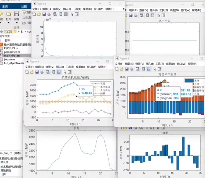
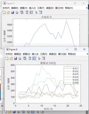
4. Optimization Results

Program outputs:

1. Convergence curve of the particle swarm optimization algorithm
2. Comparison chart of 24-hour load demand and optimized output
3. Reservoir water level change curve

Parameter Tuning Suggestions

1. Particle Swarm Parameters:

• Try different <span>numParticles</span> values (e.g., 30-100) to find a balance
• <span>w</span>, <span>c1</span>, <span>c2</span> parameters can be adjusted to balance exploration and exploitation

Cost Function Weights:

• Current weights are: 0.4 power error + 0.4 generation cost + 0.2 water level penalty
• These weight coefficients can be adjusted according to actual needs

Operational Constraints:

• Adjust <span>minPower</span> and <span>maxPower</span> to reflect actual unit capabilities
• Modify <span>minWaterLevel</span> and <span>maxWaterLevel</span> to reflect safety operating requirements

Improvement Directions

1. More Complex Hydrological Models:

• Introduce more accurate hydropower equations
• Consider factors such as terrain and pressure head

Multi-Objective Optimization:

• Set power tracking, cost control, and water level management as independent optimization objectives
• Use Pareto front methods to find optimal trade-off solutions

Hybrid Optimization Strategies:

• Combine genetic algorithms (GA) and particle swarm algorithms for hybrid optimization
• Use different algorithms at different stages to improve search efficiency

Real-Time Scheduling Expansion:

• Add a rolling window mechanism for online scheduling
• Integrate load forecasting modules for dynamic adjustments