The Wavelet Neural Network (WNN) combines wavelet analysis with neural networks, utilizing wavelet basis functions to replace the activation functions in traditional neural networks, thereby enhancing the model’s ability to handle nonlinear and non-stationary data.
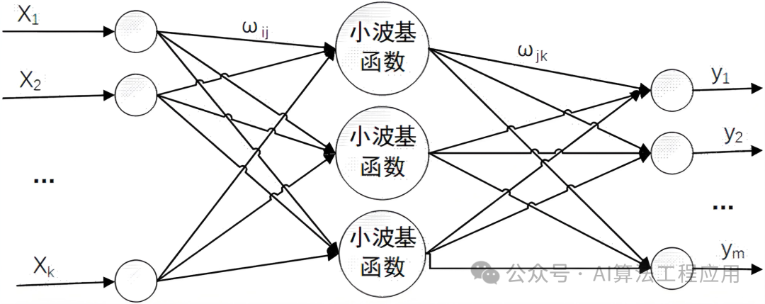
Network Structure
Assuming the input vector is and the output vector is . In the wavelet neural network, each node in the hidden layer uses a wavelet basis function , defined as:
where is the scaling factor that determines the width of the wavelet basis function; is the translation factor that determines the position of the wavelet basis function; is the time or space variable; is the mother wavelet function.
Hidden Layer Computation
For a given input , the output of the th hidden layer node can be expressed as:
Here, represents the weights connecting the input to the th hidden layer node, while is the wavelet basis function applied to the input , parameterized by the scaling factor and the translation factor .
Output Layer Computation
The output of the hidden layer is combined linearly to obtain the final network output:
where is the number of hidden layer nodes, represents the weight from the th hidden layer node to the th output node, and is the bias term.
Parameter Learning
The training of the wavelet neural network typically employs gradient descent or its variants (such as the Levenberg-Marquardt algorithm) to minimize the error between the predicted output and the target output . The error function can be defined as the mean squared error:
By adjusting all tunable parameters in the network (including weights , , and the parameters of the wavelet basis function , ), the error is minimized.
This wavelet transform-based neural network architecture fully utilizes the localization properties of wavelet transforms in the time-frequency domain while inheriting the powerful fitting capabilities of neural networks, making it suitable for complex signal processing tasks.
Data Acquisition
The data used in this article consists of short-term traffic flow data, which has been processed. For details on the data processing, please refer to previous articles on our official account: Understanding Data Preprocessing in Time Series Prediction Problems with an Example.
MATLAB Implementation Code
%% This code is for traffic flow prediction based on wavelet neural network
%% Clear environment variables
clc
clear
%% Network parameter configuration
load traffic_flux input output input_test output_test
M=size(input,2); % Number of input nodes
N=size(output,2); % Number of output nodes
n=6; % Number of hidden nodes
lr1=0.01; % Learning rate
lr2=0.001; % Learning rate
maxgen=100; % Number of iterations
% Weight initialization
Wjk=randn(n,M);Wjk_1=Wjk;Wjk_2=Wjk_1;
Wij=randn(N,n);Wij_1=Wij;Wij_2=Wij_1;
a=randn(1,n);a_1=a;a_2=a_1;
b=randn(1,n);b_1=b;b_2=b_1;
% Node initialization
y=zeros(1,N);
net=zeros(1,n);
net_ab=zeros(1,n);
% Weight learning increment initialization
d_Wjk=zeros(n,M);
d_Wij=zeros(N,n);
d_a=zeros(1,n);
d_b=zeros(1,n);
%% Input and output data normalization
[inputn,inputps]=mapminmax(input");
[outputn,outputps]=mapminmax(output");
inputn=inputn";
outputn=outputn";
error=zeros(1,maxgen);
%% Network training
for i=1:maxgen
% Accumulate error
error(i)=0;
% Loop training
for kk=1:size(input,1)
x=inputn(kk,:);
yqw=outputn(kk,:);
for j=1:n
for k=1:M
net(j)=net(j)+Wjk(j,k)*x(k);
net_ab(j)=(net(j)-b(j))/a(j);
end
temp=mymorlet(net_ab(j));
for k=1:N
y=y+Wij(k,j)*temp; % Wavelet function
end
end
% Calculate cumulative error
error(i)=error(i)+sum(abs(yqw-y));
% Weight adjustment
for j=1:n
% Calculate d_Wij
temp=mymorlet(net_ab(j));
for k=1:N
d_Wij(k,j)=d_Wij(k,j)-(yqw(k)-y(k))*temp;
end
% Calculate d_Wjk
temp=d_mymorlet(net_ab(j));
for k=1:M
for l=1:N
d_Wjk(j,k)=d_Wjk(j,k)+(yqw(l)-y(l))*Wij(l,j) ;
end
d_Wjk(j,k)=-d_Wjk(j,k)*temp*x(k)/a(j);
end
% Calculate d_b
for k=1:N
d_b(j)=d_b(j)+(yqw(k)-y(k))*Wij(k,j);
end
d_b(j)=d_b(j)*temp/a(j);
% Calculate d_a
for k=1:N
d_a(j)=d_a(j)+(yqw(k)-y(k))*Wij(k,j);
end
d_a(j)=d_a(j)*temp*((net(j)-b(j))/b(j))/a(j);
end
% Update weight parameters
Wij=Wij-lr1*d_Wij;
Wjk=Wjk-lr1*d_Wjk;
b=b-lr2*d_b;
a=a-lr2*d_a;
d_Wjk=zeros(n,M);
d_Wij=zeros(N,n);
d_a=zeros(1,n);
d_b=zeros(1,n);
y=zeros(1,N);
net=zeros(1,n);
net_ab=zeros(1,n);
Wjk_1=Wjk;Wjk_2=Wjk_1;
Wij_1=Wij;Wij_2=Wij_1;
a_1=a;a_2=a_1;
b_1=b;b_2=b_1;
end
end
%% Network prediction
% Normalize input for prediction
x=mapminmax('apply',input_test',inputps);
x=x';
yuce=zeros(92,1);
% Network prediction
for i=1:92
x_test=x(i,:);
for j=1:1:n
for k=1:1:M
net(j)=net(j)+Wjk(j,k)*x_test(k);
net_ab(j)=(net(j)-b(j))/a(j);
end
temp=mymorlet(net_ab(j));
for k=1:N
y(k)=y(k)+Wij(k,j)*temp ;
end
end
yuce(i)=y(k);
y=zeros(1,N);
net=zeros(1,n);
net_ab=zeros(1,n);
end
% Reverse normalization of predicted output
ynn=mapminmax('reverse',yuce,outputps);
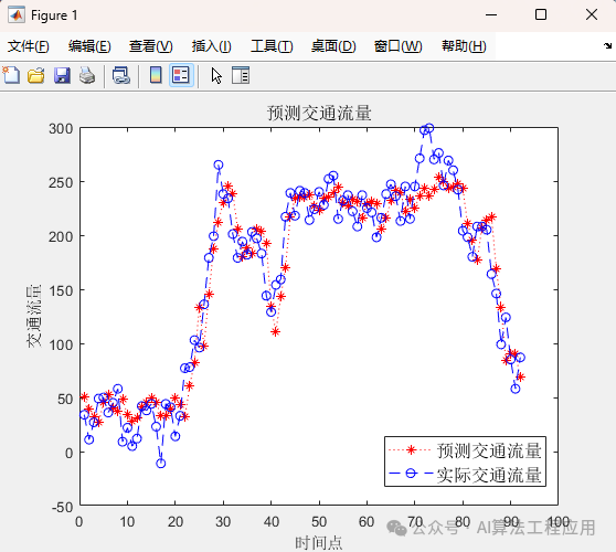
%% Result Analysis
figure(1)
plot(ynn,'r*:')
hold on
plot(output_test,'bo--')
title('Predicted Traffic Flow','fontsize',12)
legend('Predicted Traffic Flow','Actual Traffic Flow','fontsize',12)
xlabel('Time Point')
ylabel('Traffic Flow')
Function Call 1
% The two subroutines used here are:
function y=mymorlet(t)

y = exp(-(t.^2)/2) * cos(1.75*t);
Function Call 2
function y=d_mymorlet(t)

y = -1.75*sin(1.75*t).*exp(-(t.^2)/2)-t* cos(1.75*t).*exp(-(t.^2)/2) ;
Running Results
Code Acquisition
The complete executable code has been provided above. For data, please follow our official account and reply: Traffic Flow.