✅ Author Introduction: A MATLAB simulation developer passionate about research, improving both mindset and technology. For MATLAB project collaboration, feel free to contact me.
🏆 How to Obtain Code:
QQ:912100926
⛳️ Motto: A journey of a hundred miles begins with a single step.
## ⛄ 1. Introduction to CNN License Plate Recognition
1 License Plate Localization
1.1 Training Classifier
In the initial stage of preparing positive samples, the first step is to label the license plates, which involves cropping the license plate position from an image. Since training machine learning models requires a large training set, labeling the license plates must be done manually or at a cost. Fortunately, a pre-labeled dataset was found.
1.2 Coarse Localization of License Plates
Using the classifier trained in the previous step for coarse localization of the license plates.
1.3 Tilt Correction
If the license plate is not corrected for tilt, the horizontal and vertical projections, and even the rivets, cannot be processed correctly. Therefore, the first step in obtaining the license plate from vehicle information should be to check the tilt angle and perform tilt correction.
1.3.1 Calculate the Tilt Angle of the License Plate
Use a direction field-based algorithm to detect the tilt angle of the license plate.
1.3.2 Rotation
1.4 Fine Localization of License Plates
2 CNN Training
2.1 Obtain Images for Training
2.2 Build CNN Network
2.3 Execute Training
3 License Plate Recognition
3.1 Read the images obtained from fine localization in 1.4
3.2 Use the CNN trained model to recognize the fine localized images.
## ⛄ 2. Source Code
function varargout = CarId(varargin)
% CARID MATLAB code for CarId.fig
% CARID, by itself, creates a new CARID or raises the existing
% singleton*.
%
% H = CARID returns the handle to a new CARID or the handle to
% the existing singleton*.
%
% CARID(‘CALLBACK’,hObject,eventData,handles,…) calls the local
% function named CALLBACK in CARID.M with the given input arguments.
%
% CARID(‘Property’,’Value’,…) creates a new CARID or raises the
% existing singleton*. Starting from the left, property value pairs are
% applied to the GUI before CarId_OpeningFcn gets called. An
% unrecognized property name or invalid value makes property application
% stop. All inputs are passed to CarId_OpeningFcn via varargin.
%
% *See GUI Options on GUIDE’s Tools menu. Choose “GUI allows only one
% instance to run (singleton)”.
%
% See also: GUIDE, GUIDATA, GUIHANDLES
% Edit the above text to modify the response to help CarId
% Last Modified by GUIDE v2.5 04-May-2023 15:15:54
% Begin initialization code – DO NOT EDIT
gui_Singleton = 1;
gui_State = struct(‘gui_Name’, mfilename, …
‘gui_Singleton’, gui_Singleton, …
‘gui_OpeningFcn’, @CarId_OpeningFcn, …
‘gui_OutputFcn’, @CarId_OutputFcn, …
‘gui_LayoutFcn’, [] , …
‘gui_Callback’, []);
if nargin && ischar(varargin{1})
gui_State.gui_Callback = str2func(varargin{1});
end
if nargout
[varargout{1:nargout}] = gui_mainfcn(gui_State, varargin{:});
else
gui_mainfcn(gui_State, varargin{:});
end
% End initialization code – DO NOT EDIT
% — Executes just before CarId is made visible.
function CarId_OpeningFcn(hObject, eventdata, handles, varargin)
% This function has no output args, see OutputFcn.
% hObject handle to figure
% eventdata reserved – to be defined in a future version of MATLAB
% handles structure with handles and user data (see GUIDATA)
% varargin command line arguments to CarId (see VARARGIN)
% Choose default command line output for CarId
handles.output = hObject;
% Hide axes
set(handles.axes1,’visible’,’off’);
set(handles.axes2,’visible’,’off’);
set(handles.axes3,’visible’,’off’);
set(handles.axes4,’visible’,’off’);
set(handles.axes5,’visible’,’off’);
set(handles.axes6,’visible’,’off’);
set(handles.axes7,’visible’,’off’);
set(handles.axes8,’visible’,’off’);
set(handles.axes9,’visible’,’off’);
set(handles.axes10,’visible’,’off’);
set(handles.axes11,’visible’,’off’);
set(handles.axes12,’visible’,’off’);
set(handles.axes13,’visible’,’off’);
% Update handles structure
guidata(hObject, handles);
% UIWAIT makes CarId wait for user response (see UIRESUME)
% uiwait(handles.figure1);
% — Outputs from this function are returned to the command line.
function varargout = CarId_OutputFcn(hObject, eventdata, handles)
% varargout cell array for returning output args (see VARARGOUT);
% hObject handle to figure
% eventdata reserved – to be defined in a future version of MATLAB
% handles structure with handles and user data (see GUIDATA)
% Get default command line output from handles structure
varargout{1} = handles.output;
%======================my code========================%
function openLocal_Callback(hObject,eventdata,handles)
[filename, pathname]=uigetfile({‘*.jpg; *.png; *.bmp; *.tif’;’*.png’;’All Image Files’;’*.*’},’Please select image path’);
if pathname==0
return;
end
I=imread([pathname filename]);
% Display original image
axes(handles.axes1); % Set the axis with Tag value axes1 as current
imshow(I,[]); % Solve the problem of images being too large to display. Why? It seems to auto-scale.
title(‘Original Image’);
handles.I=I; % Update image
% Update handles structure
guidata(hObject, handles);
% — Executes on button press in btnGray2.
function btnGray2_Callback(hObject, eventdata, handles)
% hObject handle to btnGray2 (see GCBO)
% eventdata reserved – to be defined in a future version of MATLAB
% handles structure with handles and user data (see GUIDATA)
I=handles.chepaiyu;
I = rgb2gray(I);
axes(handles.axes8) % Set the axis with Tag value axes1 as current
imshow(I,[]); % Solve the problem of images being too large to display. Why? It seems to auto-scale.
title(‘Grayscale Processing’);
handles.gray2=I; % Update original image
% Update handles structure
guidata(hObject, handles);
% — Executes on button press in btnBalance.
function btnBalance_Callback(hObject, eventdata, handles)
% hObject handle to btnBalance (see GCBO)
% eventdata reserved – to be defined in a future version of MATLAB
% handles structure with handles and user data (see GUIDATA)
I=handles.gray2;
I = histeq(I);
axes(handles.axes9) % Set the axis with Tag value axes1 as current
imshow(I,[]); % Solve the problem of images being too large to display. Why? It seems to auto-scale.
title(‘Histogram Equalization’);
handles.balance=I; % Update original image
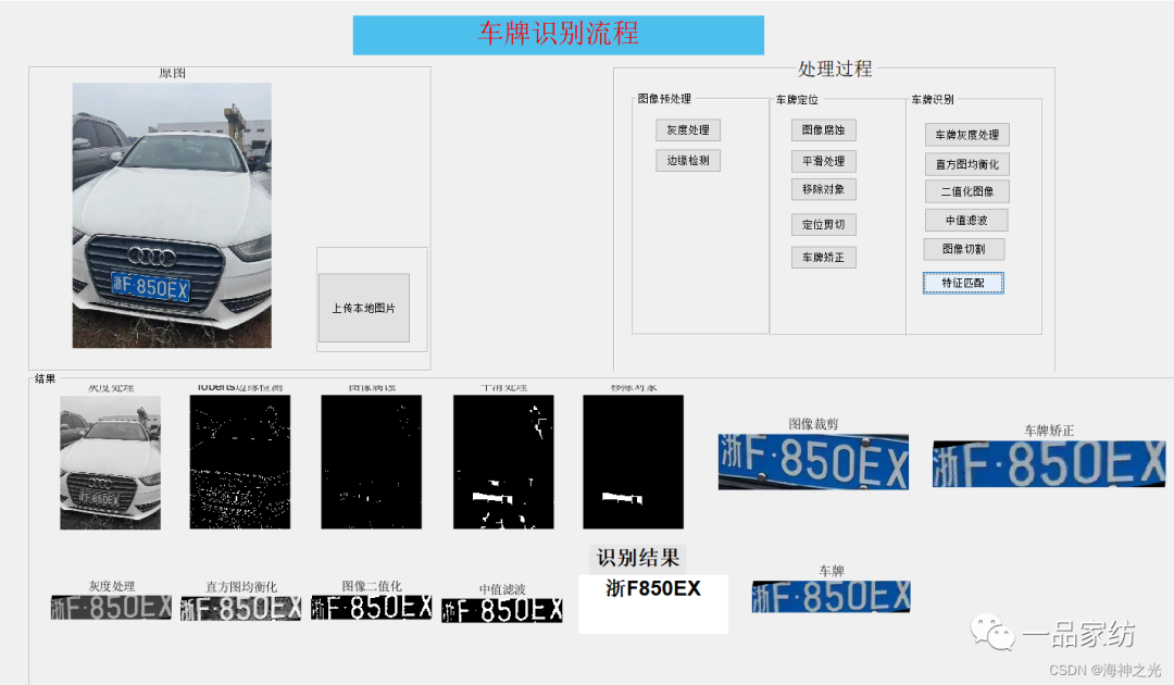
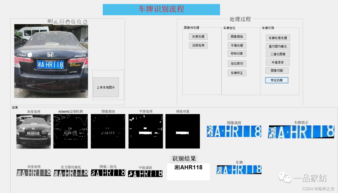
## ⛄ 3. Results
## ⛄ 4. MATLAB Version and References
**1 MATLAB Version**
2014a
**2 References**
[1] Zhang Junfeng, Shang Zhenhong, Liu Hui. Design and Implementation of License Plate Recognition System Based on Color Features and Template Matching [J]. Software Guide. 2018, 17(01)
**3 Note**
This section is extracted from the internet for reference only. If there is any infringement, please contact for removal.
**🍅 Simulation Consulting**
1 Various Intelligent Optimization Algorithm Improvements and Applications**
Production scheduling, economic scheduling, assembly line scheduling, charging optimization, workshop scheduling, departure optimization, reservoir scheduling, 3D packing, logistics site selection, cargo location optimization, bus scheduling optimization, charging pile layout optimization, workshop layout optimization, container ship loading optimization, pump combination optimization, medical resource allocation optimization, facility layout optimization, visual domain base station and drone site selection optimization.
**2 Machine Learning and Deep Learning**
Convolutional Neural Networks (CNN), LSTM, Support Vector Machines (SVM), Least Squares Support Vector Machines (LSSVM), Extreme Learning Machines (ELM), Kernel Extreme Learning Machines (KELM), BP, RBF, Wide Learning, DBN, RF, RBF, DELM, XGBOOST, TCN for wind power prediction, photovoltaic prediction, battery life prediction, radiation source identification, traffic flow prediction, load forecasting, stock price prediction, PM2.5 concentration prediction, battery health status prediction, water optical parameter inversion, NLOS signal identification, subway stop precision prediction, transformer fault diagnosis.
**3 Image Processing**
Image recognition, image segmentation, image detection, image hiding, image registration, image stitching, image fusion, image enhancement, image compressed sensing.
**4 Path Planning**
Traveling Salesman Problem (TSP), Vehicle Routing Problem (VRP, MVRP, CVRP, VRPTW, etc.), UAV 3D path planning, UAV collaboration, UAV formation, robot path planning, grid map path planning, multimodal transport problems, vehicle collaborative UAV path planning, antenna linear array distribution optimization, workshop layout optimization.
**5 UAV Applications**
UAV path planning, UAV control, UAV formation, UAV collaboration, UAV task allocation.
**6 Wireless Sensor Positioning and Layout**
Sensor deployment optimization, communication protocol optimization, routing optimization, target positioning optimization, Dv-Hop positioning optimization, Leach protocol optimization, WSN coverage optimization, multicast optimization, RSSI positioning optimization.
**7 Signal Processing**
Signal recognition, signal encryption, signal denoising, signal enhancement, radar signal processing, signal watermark embedding and extraction, electromyography signals, electroencephalography signals, signal timing optimization.
**8 Power Systems**
Microgrid optimization, reactive power optimization, distribution network reconstruction, energy storage configuration.
**9 Cellular Automata**
Traffic flow, crowd evacuation, virus spread, crystal growth.
**10 Radar**
Kalman filter tracking, track association, track fusion.