This note covers the course listened to:
Teacher Guo Yanfu on Bilibili (original version on YouTube)
“12 Statistics, 13 Regression and Interpolation”
Criticism and corrections are welcome
(1) Statistics1. Descriptive Statistics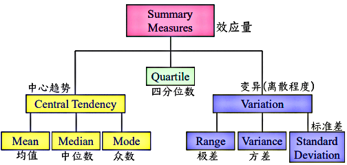 (1) Central Tendency1) Functions — Calculate xxx①mean()–Mean ②median()–Median ③mode()–Mode ④prctile()–Percentile ⑤max()–Maximum ⑥min()–Minimumeg.
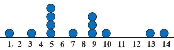
X = [1 3 5 5 5 5 7 9 9 9 10 13 14];
mean(X);    % The mean of the data is 7.3077
median(X);  % The median of the data is 7
mode(X);    % The mode of the data is 5
prctile(X, 0);        % The 0% percentile of the data is 0
prctile(X, 50); % The 50% percentile of the data is 7
prctile(X, 100); % The 100% percentile of the data is 14
prctile(X, 12.6); % The 12.6% percentile of the data is 3.2760
2) Functions — Draw statistical charts①bar()-–Bar chart ②stem()–Stem plot ③area()–Area plot ④boxplot()–Box ploteg.1. Draw bar, area, and stem plots
x = 1:14;freqy = [1 0 1 0 4 0 1 0 3 1 0 0 1 1];
subplot(1,3,1); bar(x,freqy); xlim([0 15]);
subplot(1,3,2); area(x,freqy); xlim([0 15]);
subplot(1,3,3); stem(x,freqy); xlim([0 15]);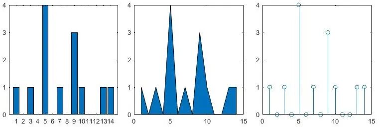 eg.2. Draw a box plot (can highlight the quartiles of the data)
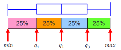
marks = [80 81 81 84 88 92 92 94 96 97];
boxplot(marks);
prctile(marks, [25 50 75]) % Get [81 90 94]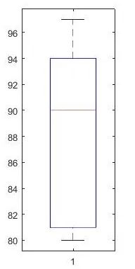 (2) Variation1) Dispersionstd()–Calculate thestandard deviationvar()–Calculate thevarianceeg.
X = [1 3 5 5 5 5 7 9 9 9 10 13 14];
std(X);    % Get 3.7944
var(X);    % Get 14.3974
2) Skewnessskewness()–Calculate the skewnessSkewness reflects the degree of symmetry of the data:When the data isleft-skewed, its skewness<0.When the data is completelysymmetrical, its skewness=0.When the data isright-skewed, its skewness>0.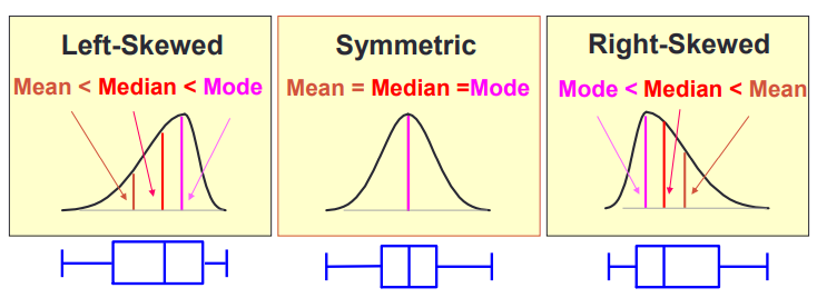 eg.
eg.
X = randn([10 3]); % Construct a 10*3 matrix X
(X(:,1)<0, 1) = 0; % Make the first column right-skewed
(X(:,3)>0, 3) = 0; % Make the second column left-skewed
boxplot(X, {'Right-skewed', 'Symmetric', 'Left-skewed'});
skewness(X); % Get [0.5162 -0.7539 -1.1234]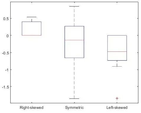 3) Kurtosiskurtosis()–Calculate the kurtosisKurtosis characterizes theheight of the peak of the probability density distribution curve at the mean.Kurtosis reflects thesharpness of the peak.
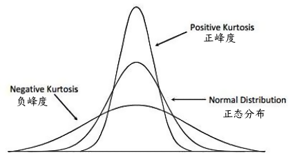 2. Inferential Statistics(1) The core of inferential statistics is hypothesis testing.(2) Functions①ttest()–T-test ③ranksum()–Rank sum test ②ztest()–Z-test ④signrank()–Sign rank testeg.
load examgrades      % Load a MAT file named examgrades
x = grades(:,1);     % Extract the first column of the grades matrix and assign it to variable x
y = grades(:,2);     % Extract the second column of the grades matrix and assign it to variable y
[h,p] = ttest(x,y);  % Get [h p] = [0 0.9805]
Indicates that at the default significance level (5%), we have no reason to reject that x and y are from the same distributionh: represents the test result.When h is 1, it means rejecting the null hypothesis at the default 5% significance level;When h is 0, it means we cannot reject the null hypothesis. p: the p-value, which reflects the probability that the observed sample difference is due to random factors.In the given example, the result is h = 0 and p = 0.9805.This indicates: Since h = 0, we cannot reject the null hypothesis at the 5% significance level. p = 0.9805, which is much greater than 0.05, indicates that the sample data does not provide sufficient evidence to reject the null hypothesis. In summary, this means that there is no significant difference in the means of the two samples x and y.(2) Fitting
※ Knowledge Supplement
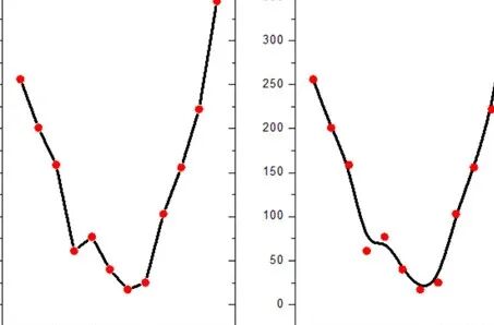
Interpolation (left)VS Fitting (right)
1. Interpolation and Fitting both belong to the function approximation problem, which establishes a continuous function based on a set of discrete data points.
1) Interpolation requires the function curve to pass through all data points;
2) Fitting does not need to pass through all points, Fitting considers the overall requirement to minimize the sum of distances from each data point to the approximating function.
2. Regression: Used to study the relationship between two or more variables.
1) If there are two variables, it is calledSimple Regression; if the relationship between the variables is linear, it is calledLinear Regression.
2) Example: When studying the relationship between drug dosage (x) and the degree of blood pressure reduction (y, treatment effect), a simple linear regression equation y=ax+b can be constructed (a is usually a positive number, indicating that the higher the dosage, the more significant the blood pressure reduction, i.e., “the more dosage, the better the effect”). By using the least squares method to fit the line, the data points and the fitted line y=ax+b can be plotted on the coordinate plane. If the data closely fits the line, it indicates a strong positive linear correlation between dosage and effect. This model can be used for prediction: given a known drug dosage x, estimate the blood pressure reduction y (e.g., “using 30mg of the drug, expect a reduction of 15mmHg”), or infer the dosage based on the target effect (e.g., “to reduce blood pressure by 20mmHg, 40mg of the drug should be used”), guiding personalized medication in clinical practice.(Note: Actual medical regression is more complex, requiring consideration of confounding factors, non-linear relationships, etc., this is a simplified example).
3. Regression and Fitting have essential differences:
| Regression | Fitting | |
|---|---|---|
| Definition | A statistical modeling method used to analyze the relationships between variables. | It is the process of approximating data points with a function, making the curve close to the observed values. |
| Application Scope | Depends on fitting techniques but is limited to statistical model construction scenarios. | Has a broader application scope, not limited to regression (e.g., mathematical interpolation, signal processing, etc.). |
| Purpose | To explain variable associations or predict dependent variables (e.g., predicting dosage – effect relationship). | Only seeks the best match between the equation/curve and the data, without focusing on the causal meaning of the variables. |
1. Polynomial Fitting
(1) Simple Polynomial Fitting
polyfit(x, y, n)–Perform n-th degree polynomial fitting on data x and y
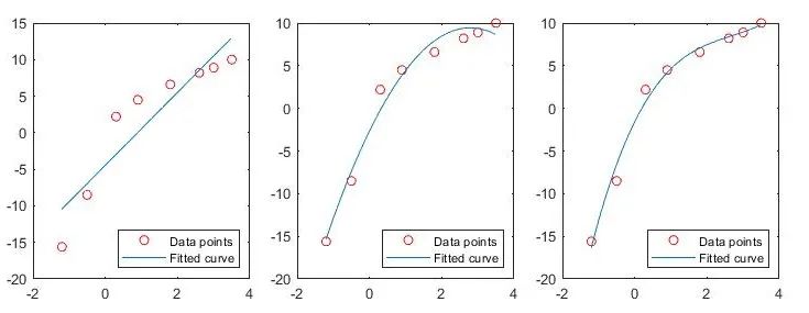
x = [-1.2 -0.5 0.3 0.9 1.8 2.6 3.0 3.5];
y = [-15.6 -8.5 2.2 4.5 6.6 8.2 8.9 10.0];
for i=1:3    % Start a loop, where the loop variable i takes values 1, 2, 3
    p = polyfit(x,y,i);    % Perform first, second, and third fitting respectively
    xfit = x(1):0.1:x(end); yfit = polyval(p,xfit);
    subplot(1,3,i); plot(x,y,'ro',xfit,yfit);
    legend('Data points','Fitted curve','Location','southeast');
end
Notes:
4 When i=1, perform first-degree polynomial fitting/linear fitting; when i=2, perform second-degree polynomial fitting, resulting in a parabola; when i=3, perform third-degree polynomial fitting.
5 Generate the fitted curve: xfit creates a vector from the first element of x to the last element, with a step of 0.1, which determines the drawing range of the fitted curve.polyval(p,xfit) calculates the function values yfit corresponding to xfit based on the previously obtained polynomial coefficients p.
6 Draw the image: subplot(1,3,i) divides the image window into 1 row and 3 columns of subplots, and selects the i-th subplot for drawing. plot(x,y,’ro’,xfit,yfit) will draw red circular points (‘ro’) to represent the original data points, while using a curve to represent the fitting result.
7 Add a legend: mark the red circular points as “Data points”, mark the fitted curve as “Fitted curve”, and place the legend in the lower right corner (‘Location’,’southeast’).
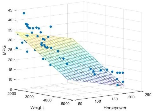
(2) Multiple Linear Fittingregress(y, X)–Perform multiple linear regression on data X and y
load carsmall;y = MPG; x1 = Weight; x2 = Horsepower;    % Import dataset
X = [ones(length(x1),1) x1 x2];        % Construct augmented X matrix
b = regress(y,X);                % Perform linear regression

x1fit = min(x1):100:max(x1); x2fit = min(x2):10:max(x2);
[X1FIT,X2FIT] = meshgrid(x1fit,x2fit);
YFIT = b(1)+b(2)*X1FIT+b(3)*X2FIT;
scatter3(x1,x2,y,'filled'); hold on;mesh(X1FIT,X2FIT,YFIT); hold off;
xlabel('Weight'); ylabel('Horsepower'); zlabel('MPG'); view(50,10);
Notes:
1 load carsmall;: Load the built-in MATLAB car dataset (including model, fuel consumption, weight, etc.)
2 y = MPG;: Set the dependent variable as “miles per gallon” (MPG, reflecting fuel efficiency);
x1 = Weight; x2 = Horsepower;: Set the independent variables as “weight” (x1) and “horsepower” (x2).
3 ones(length(x1),1): Generate a column vector of all 1s with the same length as x1 (corresponding to the intercept term in the regression equation);
[ones(length(x1),1) x1 x2]: Merge the all 1s column, x1 column, and x2 column into matrix X, shaped as [number of samples × 3].
[1, Weight₁, Horsepower₁;
1, Weight₂, Horsepower₂;
…]
4 regress(y,X): Solve the linear regression equation y = b₀ + b₁x₁ + b₂x₂ + ε, returning the coefficient vector b = [b₀, b₁, b₂]
b(1): Intercept term b₀ (the value of y when x1 and x2 are 0);
b(2): The coefficient of x1 (weight), indicating the impact of each unit increase in weight on MPG;
b(3): The coefficient of x2 (horsepower), indicating the impact of each unit increase in horsepower on MPG.
6 x1fit = min(x1):100:max(x1): Generate grid points between the minimum and maximum values of x1 (weight) with a step of 100;
x2fit = min(x2):10:max(x2): Generate grid points between the minimum and maximum values of x2 (horsepower) with a step of 10.
7 meshgrid(X1FIT,X2FIT): Convert one-dimensional vectors into two-dimensional grid matrices for subsequent surface plotting.
8 Calculate the predicted MPG values for each point based on the regression coefficients b and grid points X1FIT, X2FIT:
YFIT = b₀ + b₁×X1FIT + b₂×X2FIT.
9 scatter3(x1,x2,y,’filled’): Draw a three-dimensional scatter plot, where each point represents a car (weight → X-axis, horsepower → Y-axis, MPG → Z-axis);
10 mesh(X1FIT,X2FIT,YFIT): Draw the regression plane (fitted surface), visually showing how weight and horsepower jointly affect MPG;
hold on/off: Ensure that the scatter plot and surface are drawn in the same coordinate system.
11 xlabel, ylabel, zlabel: Add labels to the three axes;
12 view(50,10): Set the view angle to 10° elevation and 50° azimuth for better observation of the three-dimensional figure.
2. Non-linear Fitting
Enter cftool() in the command window to open the Curve Fitting Toolbox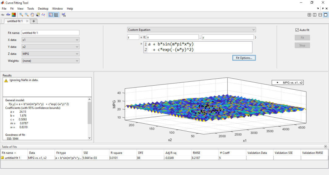 (3) Interpolation1. One-dimensional Interpolationinterp1(x,v) or interp1(x,v,xq)–Linear interpolationspline(x,v) or spline(x,v,xq)–Cubic spline interpolationpchip(x,v) or pchip(x,v,xq)–Cubic Hermite interpolationmkpp(breaks,coefs)–Generate a piecewise polynomialppval(pp,xq)–Calculate the interpolation result of the piecewise polynomial
eg.1. interp1(x, v, xq) and spline(x, v, xq). The meanings of each parameter are as follows:
x,v: Sample points to be interpolated
xq: Query points, the function returns the interpolation results at these points.
% Construct data
x = linspace(0, 2*pi, 40); x_m = x; x_m([11:13, 28:30]) = NaN; y_m = sin(x_m);
plot(x_m, y_m, 'ro', 'MarkerFaceColor', 'r'); hold on;
% Perform linear interpolation
m_i = ~isnan(x_m);y_i = interp1(x_m(m_i), y_m(m_i), x);
plot(x,y_i, '-b'); hold on;
% Perform cubic spline interpolation
m_i = ~isnan(x_m);y_i = spline(x_m(m_i), y_m(m_i), x);
plot(x,y_i, '-g');
legend('Original', 'Linear', 'Spline');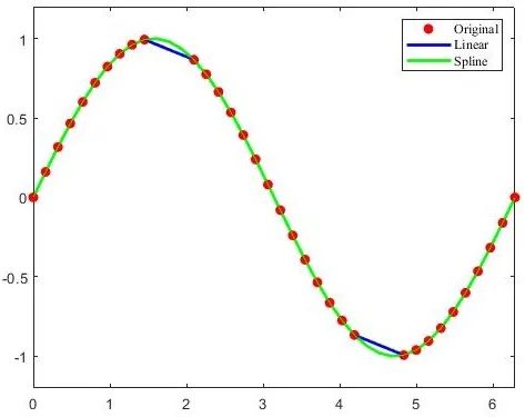 The principle of cubic spline interpolation is to use cubic function curves that are tangent to each other between every two sample points for interpolation.eg.2. If the spline() method does not specify query points, it returns a structure that encapsulates the coefficients of the interpolation cubic function.Usingmkpp(breaks, coefs) can create a similar structure,Usingppval(pp, xq) can calculate the interpolation results at the query points.
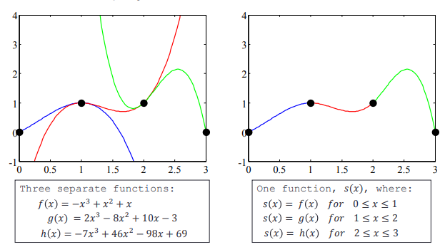 eg.3. pchip(x, y, xq) function can perform cubic Hermite interpolation, this algorithm also uses cubic functions for interpolation, but the resulting curve is smoother.
x = -3:3; y = [-1 -1 -1 0 1 1 1]; xq1 = -3:.01:3;p = pchip(x,y,xq1);s = spline(x,y,xq1);plot(x,y,'o',xq1,p,'-',xq1,s,'-.')legend('Sample Points','pchip','spline','Location','SouthEast')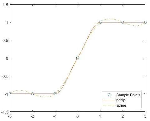
2. Two-dimensional Interpolationinterp2()–Two-dimensional interpolation (Passing a string to the method parameter can specify the interpolation algorithm)
| Interpolation Method | Description–The value inserted at the query point is based on【】 | Continuity Mark |
|---|---|---|
| ‘linear’ | 【Linear interpolation of values at neighboring grid points in each dimension】 | C0 |
| ‘spline’ | 【Cubic interpolation of values at neighboring grid points in each dimension】Interpolation based on cubic splines with non-end conditions | C2 |
| ‘nearest’ | 【The value closest to the sample grid point】 | Discontinuous |
| ‘cubic’ | 【Cubic interpolation of values at neighboring grid points in each dimension】Interpolation based on cubic convolution | C1 |
| ‘makima’ | 【Piecewise function of polynomial of degree at most 3, calculated using values of adjacent grid points in each dimension】Modified Akima cubic Hermite interpolation. To prevent overshooting, the Akima formula has been improved | C1 |
eg.
% Construct sample points
xx = -2:.5:2; yy = -2:.5:3; [x,y] = meshgrid(xx,yy);
xx_i = -2:.1:2; yy_i = -2:.1:3; [x_i,y_i] = meshgrid(xx_i,yy_i);
z = x.*exp(-x.^2-y.^2);
% Linear interpolation
subplot(1, 2, 1); z_i = interp2(xx,yy,z,x_i,y_i);surf(x_i,y_i,z_i); hold on;plot3(x,y,z+0.01,'ok','MarkerFaceColor','r'); hold on;
% Cubic interpolation
subplot(1, 2, 2); z_ic = interp2(xx,yy,z,x_i,y_i, 'spline');surf(x_i,y_i,z_ic); hold on;plot3(x,y,z+0.01,'ok','MarkerFaceColor','r'); hold on;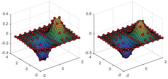
This post is a personal study note
For learning and communication purposes only
Please correct any errors
Text | Zhou Xiaoba
Images | Zhou Xiaoba, MATLAB official website