Click the “Read More” button at the bottom or reply with the keyword “code” in the backend
to download the complete program + data + instruction manual
1. Introduction to the Program and Algorithm:
Basic Content:
-
This code is compiled on the Matlab platform, combining Convolutional Neural Networks (CNN) with Bidirectional Long Short-Term Memory Networks (Bi-LSTM) for data regression prediction.
-
The training data includes 8 features and 1 response value, predicting 1 output value from 8 input values (multivariate, multi-input time series regression prediction).
-
Normalization of training data enhances network generalization.
-
Features are extracted from the data using the CNN, which are then input into the Bi-LSTM for regression prediction, improving overall network performance.
-
Train the CNN-Bi_LSTM network with customizable parameters for easy modification.
-
An optimization progress bar is automatically displayed during the iterative computation, allowing real-time monitoring of program execution.
-
Automatically outputs various error evaluation metrics and a large number of experimental result images.
Highlights and Advantages:
-
Detailed comments, with almost every key line explained, suitable for beginners.
-
Simply run the Main function to see all results, making it user-friendly.
-
Good programming practices, standardized main program structure, clear logic, and easy code readability.
-
All data is input in Excel format, making data replacement easy, suitable for lazy users.
-
Rich, detailed, and aesthetically pleasing output images for intuitive viewing of results.
-
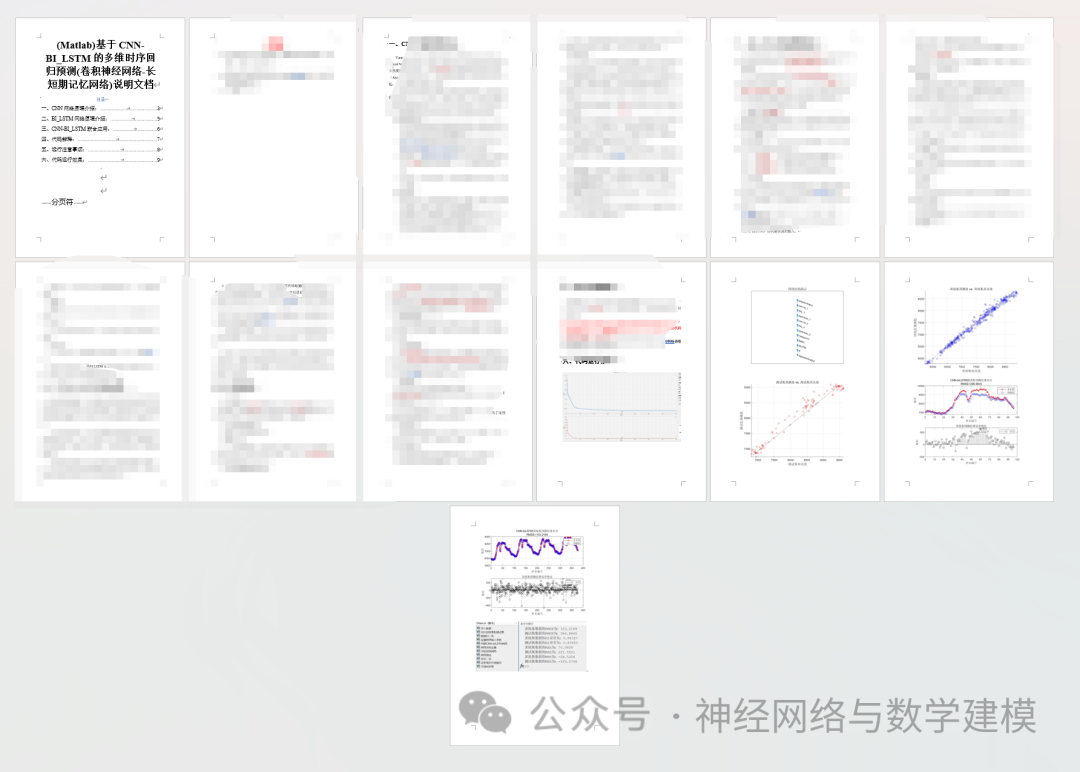
Includes a detailed instruction document (see image below), covering algorithm principles and usage instructions.
2. Actual Running Results:
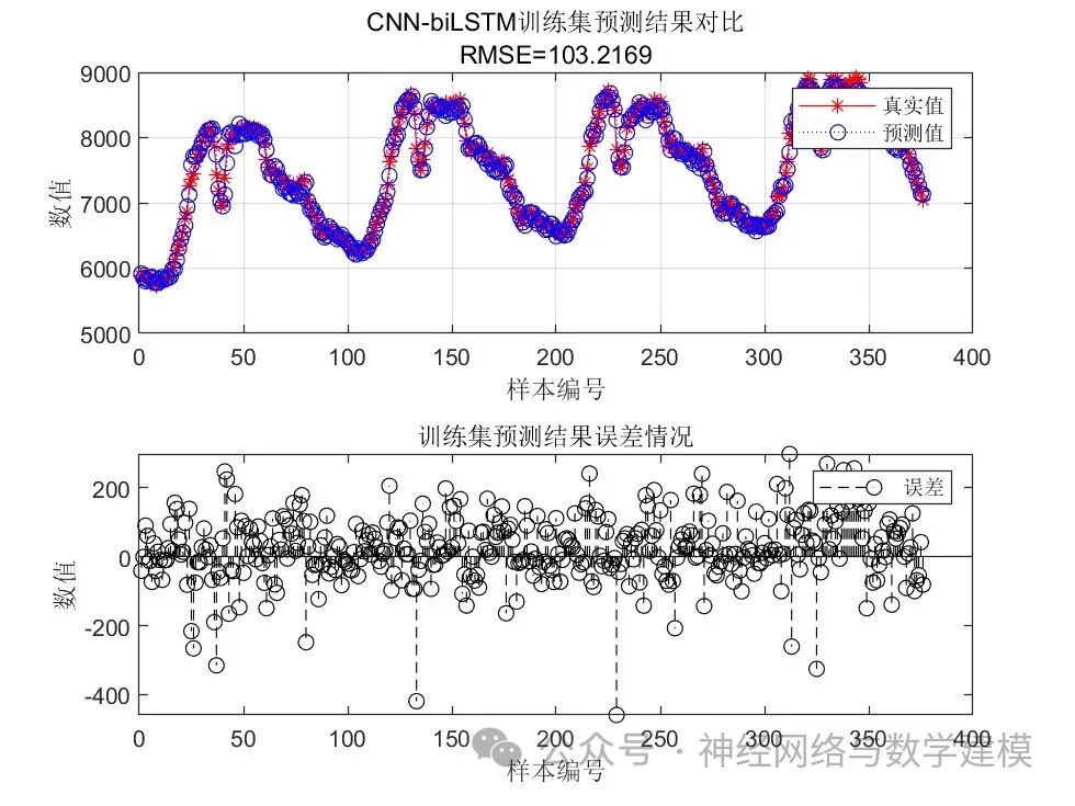
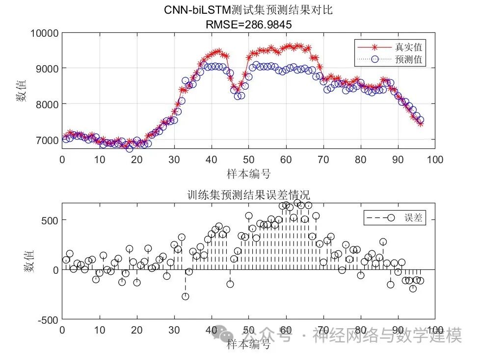
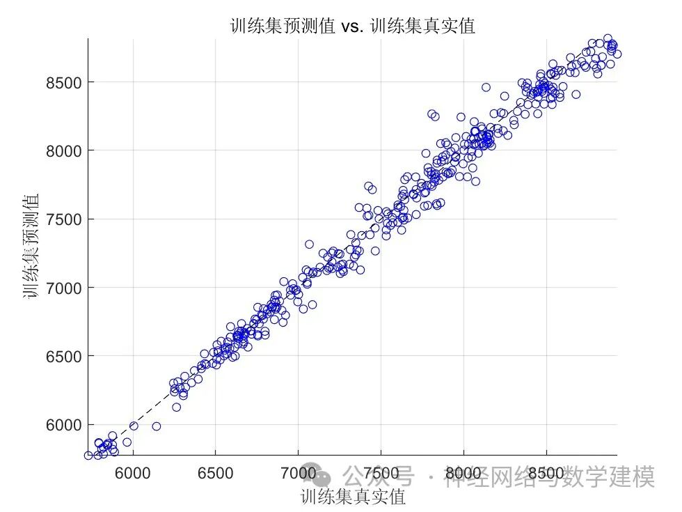
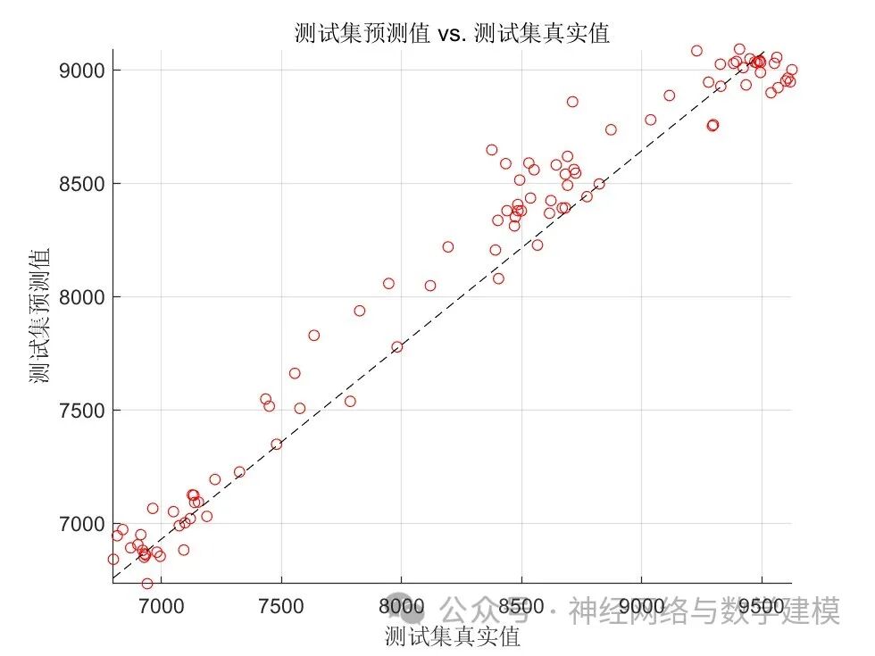
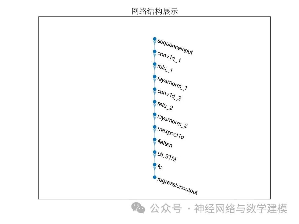
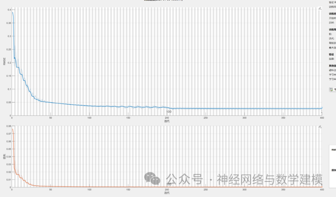
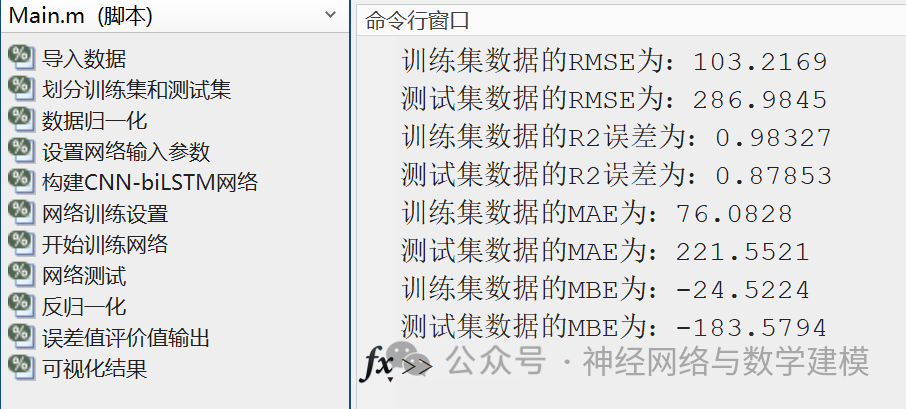
3. Part of the Program:
clc;clear;warning off;%% Import DataData = table2array(readtable("dataset.xlsx"));% This example dataset contains:% 1. A total of 472 samples (each row represents a sample)% 2. Each sample has 8 feature values (the first 8 columns represent the features, i.e., input variables)% 3. Each sample has 1 response value (the 9th column represents the response value, i.e., the predicted variable)
%% Split Training and Testing SetsInPut_num = 1:1:8; % Number of input features, the first 8 columns in the data table are input values, so set to 1:1:8, if the first 5 are inputs, set to 1:1:5OutPut_num = 9; % Number of output responses, this example has only one response value, which is the 9th in the data table, if there are multiple response values, refer to the above format for setting x:1:y
% Select the first 376 samples as the training set and the last 96 samples as the testing set, i.e., (1:376) and (377:end)Train_InPut = Data(1:376,InPut_num); % Training inputTrain_OutPut = Data(1:376,OutPut_num); % Training outputTest_InPut = Data(377:end,InPut_num); % Testing inputTest_OutPut = Data(377:end,OutPut_num); % Testing outputclear Temp;%% Data Normalization% Normalize data to the range of 0-1Temp = [Train_OutPut;Test_OutPut];[~, Ps] = mapminmax(Temp',0,1); % Normalize training input valuesSc = size(Train_InPut);Temp = reshape(Train_InPut,[1,Sc(1)*Sc(2)]);Temp = mapminmax('apply',Temp,Ps);Train_InPut = reshape(Temp,[Sc(1),Sc(2)])';% Normalize testing input valuesSc = size(Test_InPut);Temp = reshape(Test_InPut,[1,Sc(1)*Sc(2)]);Temp = mapminmax('apply',Temp,Ps);Test_InPut = reshape(Temp,[Sc(1),Sc(2)])';% Normalize training output valuesTrain_OutPut = mapminmax('apply',Train_OutPut',Ps);% Normalize testing output valuesTest_OutPut = mapminmax('apply',Test_OutPut',Ps);
4. Complete Program Download: