
Click the blue text above to follow us



Gift to readers
👨💻 Conducting research involves a profound system of thought, requiring researchers to be logical, meticulous, and serious. However, effort alone is not enough; often leveraging resources is more important than hard work. Additionally, one must have innovative and inspiring ideas. When a philosophy teacher asks you what science is or what electricity is, do not find these questions amusing. Philosophy is the mother of science; it seeks to address ultimate questions and find those self-evident questions that only children would ask but you cannot answer. It is recommended that readers browse through the content in order to avoid suddenly falling into a dark maze without finding their way back. This may not reveal all the answers to your questions, but if it can evoke clouds of doubt in your mind, it may create a beautiful sunset of thoughts. If it brings you a storm in your spiritual world, then take the opportunity to brush off the dust that has settled on your ‘lying flat’ mindset. Perhaps, after the rain, the world will be clearer…🔎🔎🔎




1 Overview
Source of literature:

Abstract: This paper investigates the inconsistency issues in EKF-based Simultaneous Localization and Mapping (SLAM) from the perspective of observability. We demonstrate through analysis that when the Jacobian matrix of the process and measurement models is evaluated at each time step based on the latest state estimate, the linearized error state system used in EKF has a higher-dimensional observable subspace than the actual nonlinear SLAM system. Consequently, the covariance estimate of EKF reduces in directions of the state space where no information is available, which is one of the main reasons for inconsistency. Based on these theoretical results, we propose a general framework for improving the consistency of EKF SLAM. In this framework, the linearization points of EKF are chosen to ensure that the resulting linearized system model has an appropriately dimensional observable subspace. We describe two algorithms that are instances of this paradigm. The first algorithm is called Observability Constraint (OC)-EKF, which selects linearization points to minimize their expected error (i.e., the difference between the linearization points and the true state) while satisfying observability constraints. The second algorithm computes the Jacobian matrix of the filter using the first available estimates of all state variables. This method is referred to as First Estimate Jacobian Matrix (FEJ)-EKF. The proposed algorithms have been tested through simulations and experiments, showing significant improvements in accuracy and consistency over standard EKF. Keywords: Simultaneous Localization and Mapping, Nonlinear Estimation, Extended Kalman Filter, Linearization Error, Estimator Inconsistency, Observability



2 Results
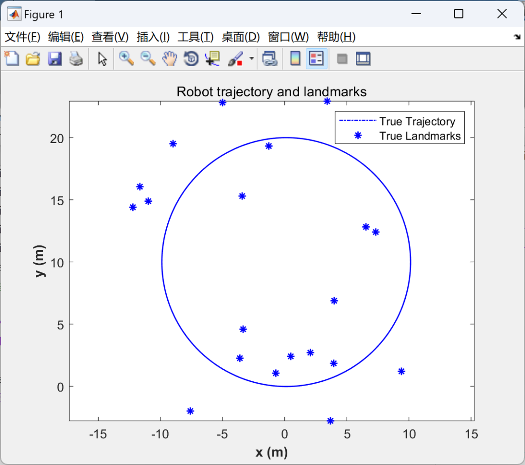
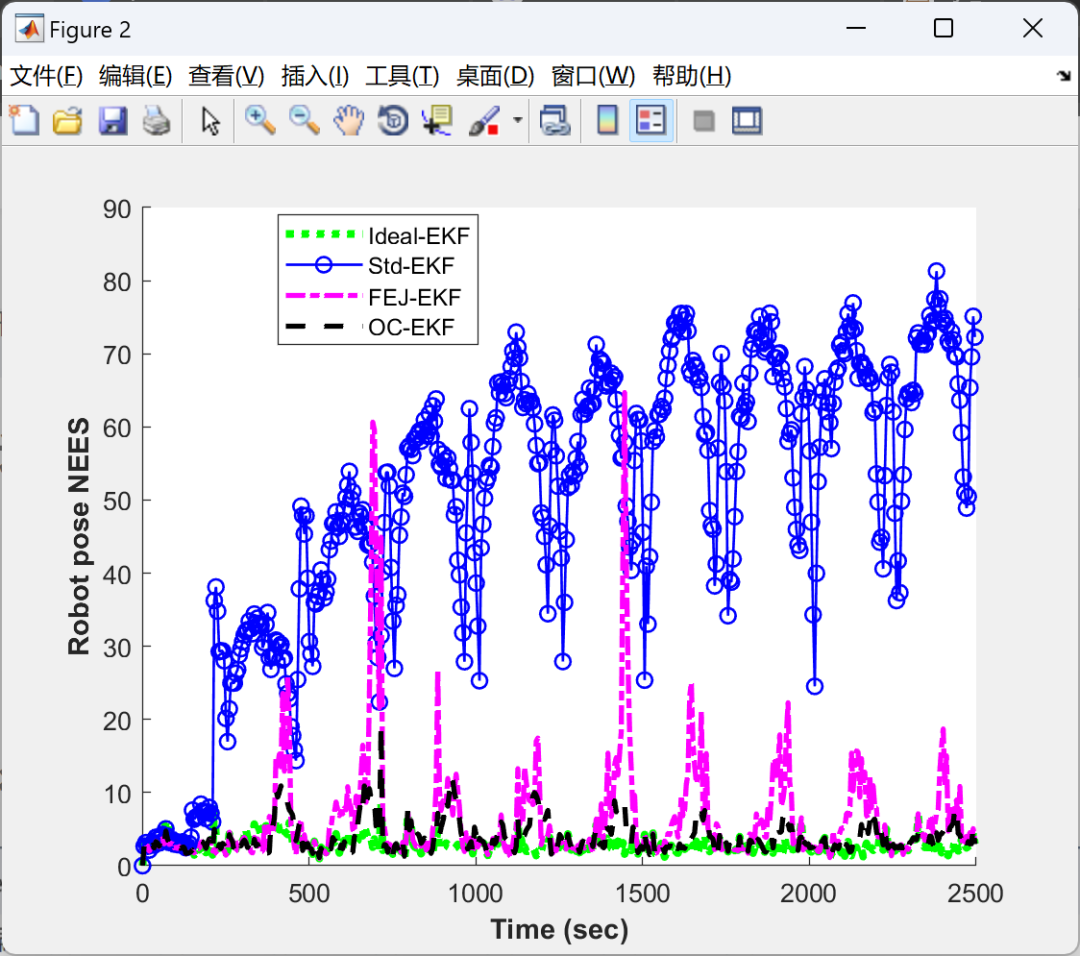
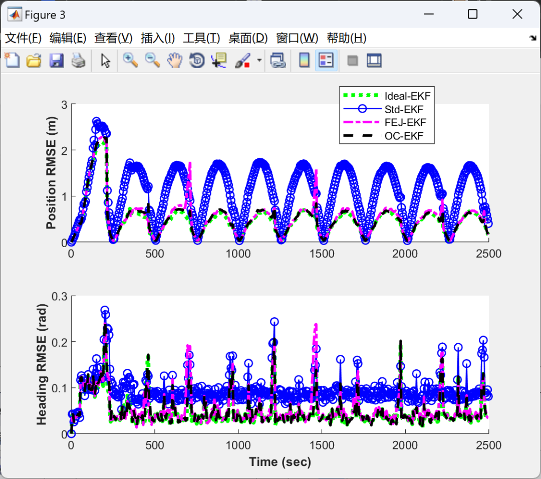
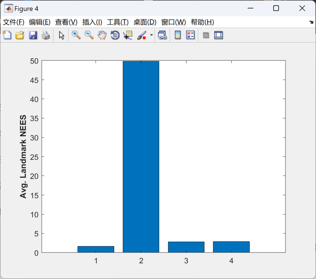
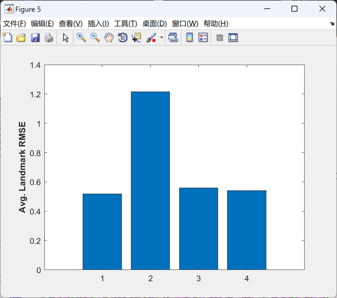
Partial code: sigma_v = sigma/sqrt(2); %.1*v_true; %sigma_w = 2*sqrt(2)*sigma; %.1*omega_true; 1*pi/180; %Q = diag([sigma_v^2 sigma_w^2]);sigma_p = .1; %noise is the percentage of distance measurement, BUT double check rws.m since sometimes we use this as a constant absolute sigmasigma_r = 1; %range measurement noisesigma_th = 10*pi/180;%bearing measurement noisenL = 20; %number of landmarks nSteps = 2500; %number of time steps nRuns = 5; %number of Monte Carlo runs if nL==1 max_range = 200;%always observe this landmark else max_range = 5;%env_size/10;%.5*v_true/omega_true;%end min_range = .5; init_steps = 0;%3 max_delay = 10;%for delayed initial NIncr = 0; %increment number of incremental MAP: 0 - not running %% preallocate memory for saving results % Ideal EKFxRest_id = zeros(3,nSteps,nRuns); %estimated trajxRerr_id = zeros(3,nSteps,nRuns); %all err statePrr_id = zeros(3,nSteps,nRuns); %actually diag of PrrneesR_id = zeros(1,nSteps,nRuns); %nees (or Mahalanobis distance) rmsRp_id = zeros(1,nSteps,nRuns); %rms of robot position rmsRth_id = zeros(1,nSteps,nRuns); %rms of robot orientation xLest_id = zeros(2,nL,nSteps,nRuns); xLerr_id = zeros(2,nL,nSteps,nRuns); Pll_id = zeros(2,nL,nSteps,nRuns); neesL_id = zeros(1,nL,nSteps,nRuns); rmsL_id = zeros(1,nL,nSteps,nRuns); nees_id = zeros(1,nSteps,nRuns); %nees for the whole state % Standard EKFxRest_std = zeros(3,nSteps,nRuns); %estimated trajxRerr_std = zeros(3,nSteps,nRuns); %all err statePrr_std = zeros(3,nSteps,nRuns); %actually diag of PrrneesR_std = zeros(1,nSteps,nRuns); %nees (or Mahalanobis distance) rmsRp_std = zeros(1,nSteps,nRuns); %rms of robot position rmsRth_std = zeros(1,nSteps,nRuns); %rms of robot orientation xLest_std = zeros(2,nL,nSteps,nRuns); xLerr_std = zeros(2,nL,nSteps,nRuns); Pll_std = zeros(2,nL,nSteps,nRuns); neesL_std = zeros(1,nL,nSteps,nRuns); rmsL_std = zeros(1,nL,nSteps,nRuns); nees_std = zeros(1,nSteps,nRuns); %nees for the whole state kld_std = zeros(1,nSteps,nRuns); % KLD % FEJ-EKFxRest_fej = zeros(3,nSteps,nRuns); %estimated trajxRerr_fej = zeros(3,nSteps,nRuns); %all err statePrr_fej = zeros(3,nSteps,nRuns); %actually diag of PrrneesR_fej = zeros(1,nSteps,nRuns); %nees (or Mahalanobis distance) rmsRp_fej = zeros(1,nSteps,nRuns); %rms of robot position rmsRth_fej = zeros(1,nSteps,nRuns); %rms of robot orientation xLest_fej = zeros(2,nL,nSteps,nRuns); xLerr_fej = zeros(2,nL,nSteps,nRuns); Pll_fej = zeros(2,nL,nSteps,nRuns); neesL_fej = zeros(1,nL,nSteps,nRuns); rmsL_fej = zeros(1,nL,nSteps,nRuns); nees_fej = zeros(1,nSteps,nRuns); %nees for the whole state kld_fej = zeros(1,nSteps,nRuns); % KLD % OC-EKFxRest_ocekf_1 = zeros(3,nSteps,nRuns); %estimated trajxRerr_ocekf_1 = zeros(3,nSteps,nRuns); %all err statePrr_ocekf_1 = zeros(3,nSteps,nRuns); %actually diag of PrrneesR_ocekf_1 = zeros(1,nSteps,nRuns); %nees (or Mahalanobis distance) rmsRp_ocekf_1 = zeros(1,nSteps,nRuns); %rms of robot position rmsRth_ocekf_1 = zeros(1,nSteps,nRuns); %rms of robot orientation xLest_ocekf_1 = zeros(2,nL,nSteps,nRuns); xLerr_ocekf_1 = zeros(2,nL,nSteps,nRuns); Pll_ocekf_1 = zeros(2,nL,nSteps,nRuns); neesL_ocekf_1 = zeros(1,nL,nSteps,nRuns); rmsL_ocekf_1 = zeros(1,nL,nSteps,nRuns); nees_ocekf_1 = zeros(1,nSteps,nRuns); %nees for the whole state kld_ocekf_1 = zeros(1,nSteps,nRuns); % KLD %% LANDMARK GENERATION: same landmarks in each run if nL==1 xL_true_fixed = [0;v_true/omega_true]; elseif nL==2 xL_true_fixed = [5 -5; 5 15]; else xL_true_fixed = gen_map(nL,v_true,omega_true,min_range, max_range, nSteps,dt); %max_range=5 end %% Monte Carlo Simulations for kk = 1:nRuns kk % % real world simulation data % % xL_true(:,:,kk) = xL_true_fixed; [v_m,omega_m, v_true_all,omega_true_all, xR_true(:,:,kk), z,R] = rws(nSteps, dt,v_true,omega_true,sigma_v,sigma_w,sigma_r,sigma_th,sigma_p,xL_true(:,:,kk),max_range,min_range); % % INITIALIZATION x0 = zeros(3,1); if init_steps P0 = zeros(3); else P0 = diag([(.0001)^2,(.0001)^2,(.0001)^2]); end for k=1:init_steps [x0,P0] = propagate_std(x0,P0,dt,v_m(k),omega_m(k),sigma_v,sigma_w); end % Ideal EKF xe_id = x0; Pe_id = P0; V_id = []; % Standard EKF xe_std = x0; Pe_std = P0; V_std = []; % FEJ-EKF xe_fej = x0; Pe_fej = P0; xL_fej_1 = []; xR_fej_k_k1 = xe_fej(1:3,1); PHI_mult_fej = eye(1); %propagation Jacobian product V_fej = []; % OC-EKF xe_ocekf_1 = x0; Pe_ocekf_1 = P0; xL_ocekf_1_1 = []; xR_oc_k_k1_1 = xe_ocekf_1(1:3,1); dpR_star_prev_1 = zeros(2,1); pR_star_prev = x0(1:2,1); dpR_ocekf_1 = zeros(2,1); V_ocekf_1 = []; PHI_mult_ocekf_1 = eye(1); lambda_1 = zeros(2,nL); % list of landmark ids that sequentially appear in the state vector lm_seq_id = []; lm_seq_std = []; lm_seq_fej = []; lm_seq_ocekf_1 = [];

3References
Some content in this article is sourced from the internet, and references will be noted. If there are any inaccuracies, please feel free to contact us for removal.




4 MATLAB Code and Articles
For more resources, including MATLAB, Simulink, and Python, please follow us for additional benefits.