
In fields such as wireless communication, digital audio, and radar systems, we often face a dilemma: we want to ensure accuracy with high sampling rates during signal acquisition, but we also need low rates during processing to reduce costs.
Multirate Signal Processing is the “variable speed engine” that resolves this dilemma. It achieves a balance between efficiency and performance by flexibly adjusting the signal sampling rate.
Single-rate refers to a system where there is only one data rate throughout the entire signal processing system;
Multirate means that there are multiple data rates within the signal processing system. By using multirate signal processing, we can save storage space, reduce communication data volume, decrease computational load, and lower design complexity.
An important application of multirate signal processing in wireless communication is in Software Defined Radio (SDR) for Digital Up Conversion (DUC) and Digital Down Conversion (DDC).
SDR faces conflicting sampling rate requirements:Signal acquisition requires a high sampling rate to reduce ADC noise and enable software processing, resulting in a very high signal rate;Signal processing and encoding expect a low rate to focus on the effective frequency band; whileDAC conversion again requires a high sampling rate to reconstruct the signal and improve the signal-to-noise ratio. Multirate signal processing technology achieves flexible signal rate conversion through interpolation and decimation, effectively integrating these requirements.
1. Core Principle: The Game Between Time Domain and Frequency Domain
The essence of multirate signal processing is to change the signal rate through Decimation (reducing the sampling rate) and Interpolation (increasing the sampling rate), supplemented by filter banks to eliminate aliasing effects.
1. Decimation (Downsampling)
Input signal data is taken every N-1 samples, and the extracted data is sorted sequentially. This process is called N-fold decimation, reducing the sampling rate to 1/N of the original.
To reduce the sampling rate by an integer factor (e.g., 2-fold decimation), a low-pass filter must first limit the signal bandwidth (e.g., to 1/2 of the Nyquist frequency).
To avoid spectral aliasing in the decimated signal, the sampling rate after decimation must still satisfy the Nyquist sampling theorem.
Input analog signals converted by high-speed ADC introduce white noise, so anti-aliasing filtering is generally required before decimation.

2. Interpolation (Upsampling)
Input signal data, insert I-1 zero values between adjacent data points, and then perform low-pass filtering. This process is called I-fold interpolation, and the sampling rate is correspondingly increased to I times the original.
As long as the passband of the low-pass filter (LPF) covers the effective bandwidth of the signal, even if the interpolation operation only inserts zero values (rather than actual sample points), an equivalent I-fold interpolation effect can still be achieved.
When the signal processed by interpolation is output through the DAC, the high-frequency noise introduced will be lower than that of the non-interpolated case.
After inserting zero values between adjacent sample points, the waveform is smoothed through a low-pass filter (for example, CD audio is upsampled from 44.1kHz to 176.4kHz to simplify DAC design).

3. Non-integer Rate Conversion
In practical applications, the rate conversion often does not have an integer relationship.
This can be achieved by first performing I-fold interpolation, then D-fold decimation, to achieve a sampling rate conversion of rational ratio (I/D) data rate.
At this time, a single low-pass filter (LPF) can be shared, with the cutoff frequency taken as the minimum of the effective bandwidth of the interpolated signal and the decimated signal.

4. Noble Identity
In multistage systems that include linear systems, interpolators, and decimators, the order of these three components can be exchanged, significantly reducing computational complexity (e.g., polyphase structures).
A simple block diagram of a multirate signal processing system is shown below:

For example, the digital down conversion (DDC) link in software-defined radio consists of a CIC filter, half-band filter (HB), and FIR filter, progressively reducing the data rate.
5. Spectral Aliasing
Assuming that in a certain system, the analog signal only has signals in the 0~2 kHz frequency band, and AD sampling is performed at a frequency of 6 kHz, then the sampled signal does not exhibit spectral aliasing, with a spectral period of 6 kHz, as shown in Figure 6-5 (a).
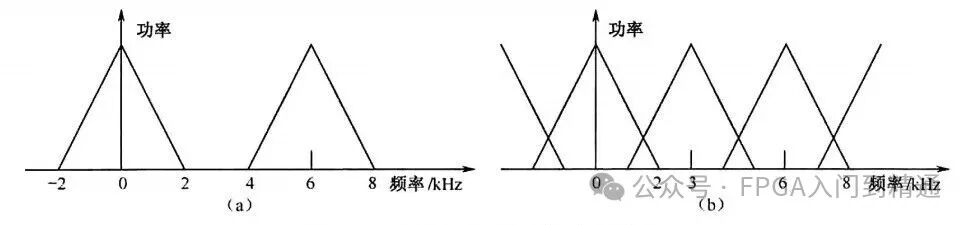
If the 6 kHz signal is directly subjected to 2-fold decimation, the spectral period of the decimated signal drops to 3 kHz. The spectral shape remains unchanged, but the period is shortened, leading to spectral aliasing, as shown in Figure 6-5 (b).
The reason for aliasing can also be understood from the perspective of the sampling theorem. The sampling frequency of the decimated signal is 3 kHz, while the highest frequency of the original analog signal is 2 kHz, which clearly does not satisfy the condition for alias-free sampling, making frequency aliasing inevitable.
Therefore, to recover the original analog signal without distortion, it is necessary to perform “anti-aliasing filtering” (i.e., low-pass filtering) before decimation, limiting the signal bandwidth to above half of the sampling frequency (to satisfy the sampling theorem).
2. MATLAB Simulation
Implementing decimation and interpolation in MATLAB is straightforward.
1. Decimation
f = 100; % Signal frequency is 100Hz
Fs = 10000; % Sampling frequency is 10KHz
% Generate sine wave
t = 0 : 1 / Fs : 0.5;c = 2 * pi * f * t;si=sin(c); % Decimation D=8; % Decimation factor d2 = si(1 : D : length(t)); % Decimation
2. Interpolation
f = 100; % Signal frequency is 100Hz
Fs = 10000; % Sampling frequency is 10KHz
% Generate sine wave
t = 0 : 1/Fs : 0.5;
c = 2 * pi * f * t;
si = sin(c);
% Interpolation
I = 8; % Interpolation factor
Isi = zeros(1, length(si)*I); % First construct a zero sequence
Isi(1 : I : length(Isi)) = si; % Insert source signal
 If you need more learning materials and source code, and want to learn FPGA practical entry and advanced topics, please read the following article: Is FPGA practical entry really difficult? Look here to avoid detours and pitfalls.
Previous readings:
Summary of the “FPGA Basics” series tutorials
Summary of commonly used techniques in Vivado
Summary of FPGA timing constraint articles
Summary of FPGA book series
Summary of FPGA advanced series articles
Summary of FPGA image processing column series
How to prepare for FPGA written and interview? (with interview questions download)