First, the raw vibration signals are preprocessed, including signal segmentation, normalization, and feature extraction, from which 11 statistical features are extracted in both time and frequency domains. Then, the multi-sensor system is modeled as a graph structure, where sensors are represented as nodes and the physical connections between sensors are represented as edges, with the correlation of sensor signals calculated as edge weights.The core algorithm employs a Spatio-Temporal Graph Neural Network (ST-GNN), combined with Long Short-Term Memory (LSTM) networks for temporal feature learning and Graph Attention Networks (GAT) for spatial feature fusion, fully utilizing the spatio-temporal dependencies between sensors.The system adopts a hybrid load training strategy, training on data from 0, 1, and 2 HP loads, and testing on unseen 3 HP load data to evaluate the model’s generalization capability. Hyperparameter optimization is performed using Optuna, achieving superior performance in the bearing fault classification task, particularly demonstrating good robustness under unknown operating conditions.
Raw vibration signal acquisition ↓Signal preprocessing and segmentation ↓Time and frequency domain feature extraction ↓Construct sensor graph structure ↓Spatio-Temporal Graph Neural Network processing ├── Temporal feature learning (LSTM) └── Spatial feature fusion (GAT) ↓Graph-level feature pooling ↓Fault classification output ↓Performance evaluation and visualizationDetailed algorithm steps:
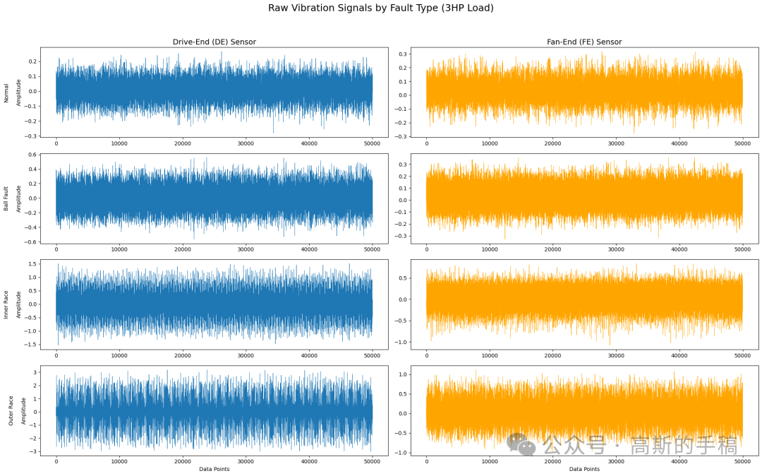
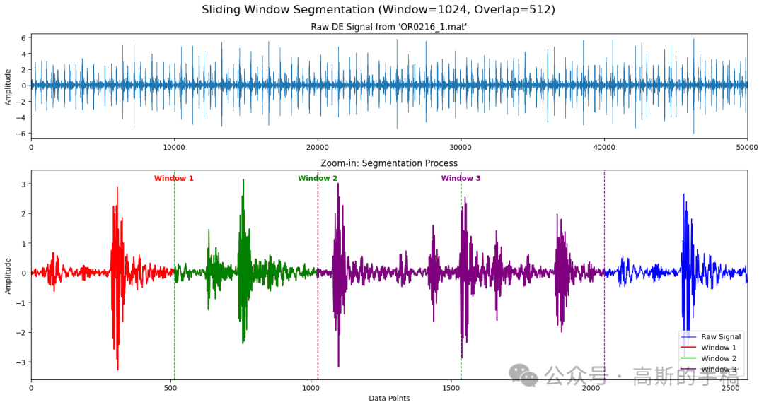
Step 1, Data preparation and preprocessing phase: Load the Case Western Reserve University bearing dataset, segment the raw vibration signals into windows of 1024 data points with a 50% overlap to increase the number of training samples. Normalize the signals to eliminate dimensional effects.
Step 2, Feature engineering phase: Extract 6 time-domain statistical features (mean, root mean square, skewness, kurtosis, peak-to-peak value, peak factor) and 5 frequency-domain features (average energy of five frequency bands) from each signal segment, constructing an 11-dimensional feature vector as the initial feature representation of the nodes.
Step 3, Graph structure construction phase: Model the two sensors at the drive end and fan end as two nodes in the graph structure, establishing edge relationships based on physical connections, and calculating the Pearson correlation coefficient between the two sensor signals as edge weights, reflecting the strength of the correlation between sensors.
Step 4, Model architecture design phase: Construct the Spatio-Temporal Graph Neural Network, first using the LSTM network to independently learn the temporal features of each sensor, capturing temporal dependencies; then aggregate the features of the two sensor nodes through the Graph Attention Network to achieve spatial information fusion.
Step 5, Training optimization phase: Employ a hybrid load training strategy, using data from 0, 1, and 2 HP loads for training, while reserving 3 HP load data as the test set. Utilize the Optuna framework for automated hyperparameter search to find optimal configurations for learning rate, dropout rate, and other parameters.
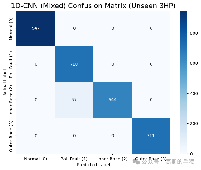
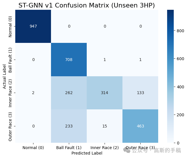
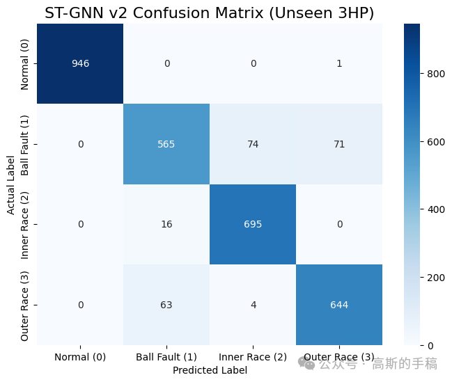
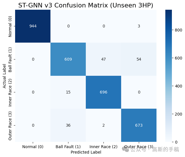
Step 6, Evaluation and analysis phase: Test the model performance on unseen 3 HP load data, calculating metrics such as accuracy, precision, recall, and F1 score, generating confusion matrices and classification reports to comprehensively evaluate the model’s generalization capability and robustness under unknown operating conditions.
Code can be referenced appropriately.
# Import necessary libraries
import torch
import torch.nn.functional as F
from torch.nn import LSTM, Linear, BatchNorm1d, Dropout
from torch_geometric.nn import GATConv, global_mean_pool
from torch_geometric.data import Data
from torch_geometric.loader import DataLoader
from torchinfo import summary
import optuna  # For hyperparameter optimization
import numpy as np
import scipy.io
import scipy.stats
from scipy.stats import pearsonr
import os
import time
import pandas as pd
import matplotlib.pyplot as plt
import seaborn as sns
from sklearn.model_selection import train_test_split
from sklearn.preprocessing import StandardScaler
from sklearn.metrics import confusion_matrix, classification_report
from skrebate import ReliefF  # For feature selection

# Configure parameters
WINDOW_SIZE = 1024  # Size of each signal segment (1024 data points)
OVERLAP = 512       # Overlap rate between segments 50%
DATA_DIR = 'cwru'  # Data directory
BATCH_SIZE = 64     # Batch size
RANDOM_STATE = 42   # Random seed
N_FEATURES = 11     # 6 time-domain features + 5 frequency-domain features

# Select device (GPU or CPU)
device = torch.device('cuda' if torch.cuda.is_available() else 'cpu')
criterion = torch.nn.CrossEntropyLoss()  # Loss function
print(f"Libraries imported successfully.")
print(f"Using device: {device}")

# Define file label mappings under different load conditions
# 0 HP load
LABEL_MAPPING_0HP = {    'Normal_0.mat': 0, 'B007_0.mat': 1, 'B014_0.mat': 1, 'B021_0.mat': 1,    'IR007_0.mat': 2, 'IR014_0.mat': 2, 'IR021_0.mat': 2,    'OR0076_0.mat': 3, 'OR0146_0.mat': 3, 'OR0216_0.mat': 3}
# 1 HP load
LABEL_MAPPING_1HP = {    'Normal_1.mat': 0, 'B007_1.mat': 1, 'B014_1.mat': 1, 'B021_1.mat': 1,    'IR007_1.mat': 2, 'IR014_1.mat': 2, 'IR021_1.mat': 2,    'OR0076_1.mat': 3, 'OR0146_1.mat': 3, 'OR0216_1.mat': 3}
# 2 HP load  LABEL_MAPPING_2HP = {    'Normal_2.mat': 0, 'B007_2.mat': 1, 'B014_2.mat': 1, 'B021_2.mat': 1,    'IR007_2.mat': 2, 'IR014_2.mat': 2, 'IR021_2.mat': 2,    'OR0076_2.mat': 3, 'OR0146_2.mat': 3, 'OR0216_2.mat': 3}
# 3 HP load (unseen test set)
LABEL_MAPPING_3HP = {    'Normal_3.mat': 0, 'B007_3.mat': 1, 'B014_3.mat': 1, 'B021_3.mat': 1,    'IR007_3.mat': 2, 'IR014_3.mat': 2, 'IR021_3.mat': 2,    'OR0076_3.mat': 3, 'OR0146_3.mat': 3, 'OR0216_3.mat': 3}
# Merge all label mappings
ALL_LABEL_MAPPINGS = {**LABEL_MAPPING_0HP, **LABEL_MAPPING_1HP, **LABEL_MAPPING_2HP, **LABEL_MAPPING_3HP}
CLASS_NAMES = ["Normal (0)", "Ball Fault (1)", "Inner Race Fault (2)", "Outer Race Fault (3)"]
num_classes = len(set(ALL_LABEL_MAPPINGS.values()))
print(f"Label mappings defined for all 4 loads (0, 1, 2, 3 HP).")
print(f"Total number of classes: {num_classes}")
def segment_signal(signal, window_size, overlap):
    """Segment 1D signal into overlapping windows."""
    segments = []
    step = window_size - overlap
    for i in range(0, len(signal) - window_size + 1, step):
        segments.append(signal[i:i + window_size])
    return np.array(segments)
def extract_time_features(segment):
    """Extract a set of statistical time-domain features from a signal segment."""
    mean = np.mean(segment)  # Mean
    rms = np.sqrt(np.mean(segment**2))  # Root mean square
    skewness = scipy.stats.skew(segment)  # Skewness
    kurt = scipy.stats.kurtosis(segment)  # Kurtosis
    p2p = np.ptp(segment)  # Peak-to-peak value
    # Peak factor: Peak / RMS
    crest_factor = (np.max(np.abs(segment)) / rms) if rms > 1e-6 else 0
    return [mean, rms, skewness, kurt, p2p, crest_factor]
def extract_freq_features(segment, n_bands=5):
    """Extract frequency domain features (band energy) from a signal segment."""
    N = len(segment)
    # Calculate FFT
    fft_vals = np.fft.fft(segment)
    fft_mag = np.abs(fft_vals)[:N // 2] * 2 / N  # Get magnitude of positive frequencies
    # Divide spectrum into n_bands frequency bands
    band_energies = []
    band_size = len(fft_mag) // n_bands
    for i in range(n_bands):
        start = i * band_size
        end = (i + 1) * band_size if i < n_bands - 1 else len(fft_mag)
        # Calculate average energy in the frequency band
        band_energy = np.mean(fft_mag[start:end])
        band_energies.append(band_energy)
    return band_energies
def extract_all_features(segment):
    """Combine time-domain and frequency-domain features for a single segment."""
    time_feats = extract_time_features(segment)  # Extract time-domain features
    freq_feats = extract_freq_features(segment, n_bands=5)  # Extract frequency-domain features
    # Concatenate all features
    return np.concatenate([time_feats, freq_feats])
# Define global edge index (connections between two sensor nodes)
edge_index_global = torch.tensor([[0, 1], [1, 0]], dtype=torch.long)
def create_graph_list_features_weighted(file_list, data_dir, label_mapping, scaler_de, scaler_fe):
    """Create a list of PyG data objects for feature + weighted model."""
    all_data_list = []
    for file_name in file_list:
        file_path = os.path.join(data_dir, file_name)
        if not os.path.exists(file_path): continue
        label = label_mapping[file_name]
        mat_data = scipy.io.loadmat(file_path)
        de_key = [key for key in mat_data.keys() if 'DE_time' in key][0]
        fe_key = [key for key in mat_data.keys() if 'FE_time' in key][0]
        de_signal_full = mat_data[de_key].flatten()
        fe_signal_full = mat_data[fe_key].flatten()
        min_len = min(len(de_signal_full), len(fe_signal_full))
        de_signal_full, fe_signal_full = de_signal_full[:min_len], fe_signal_full[:min_len]
        # Calculate Pearson correlation between the two sensor signals as edge weights
        corr, _ = pearsonr(de_signal_full, fe_signal_full)
        edge_weight_val = abs(corr) + 1e-6  # Take absolute value and add small value to avoid zero
        edge_weight = torch.tensor([edge_weight_val, edge_weight_val], dtype=torch.float)
        # Segment signals
        de_segments_raw = segment_signal(de_signal_full, WINDOW_SIZE, OVERLAP)
        fe_segments_raw = segment_signal(fe_signal_full, WINDOW_SIZE, OVERLAP)
        if de_segments_raw.size > 0:
            # Normalize signal segments
            de_segments_norm = scaler_de.transform(de_segments_raw)
            fe_segments_norm = scaler_fe.transform(fe_segments_raw)
            for i in range(len(de_segments_norm)):
                # Extract features
                de_feats = extract_all_features(de_segments_norm[i])
                fe_feats = extract_all_features(fe_segments_norm[i])
                # Create node feature tensor
                x = torch.tensor([de_feats, fe_feats], dtype=torch.float)
                y = torch.tensor([label], dtype=torch.long)
                # Create graph data object
                graph_data = Data(x=x, edge_index=edge_index_global, y=y, edge_weight=edge_weight)
                all_data_list.append(graph_data)
    print(f"Loaded {len(all_data_list)} weighted feature samples from {len(file_list)} files.")
    return all_data_list
# Define Spatio-Temporal Graph Neural Network model (ST-GNN v3)
class ST_GNN_v3_w(torch.nn.Module):
    """ST-GNN v3 model (LSTM -> GAT + features + weights)"""
    def __init__(self, num_nodes, feature_length, rnn_hidden_size, gnn_hidden_size, num_classes, dropout_rate, heads=2):
        super(ST_GNN_v3_w, self).__init__()
        self.num_nodes = num_nodes  # Number of nodes (sensors)
        self.feature_length = feature_length  # Feature length
        self.rnn_hidden_size = rnn_hidden_size  # LSTM hidden layer size
        self.gnn_heads = heads  # Number of GAT heads
        self.gnn_out_features = gnn_hidden_size * self.gnn_heads  # Number of GAT output features
        self.input_bn = BatchNorm1d(num_nodes)  # Input batch normalization
        # 1. Temporal module (LSTM)
        self.temporal_module = LSTM(
            input_size=self.feature_length,  # Input size is feature length
            hidden_size=rnn_hidden_size,     # LSTM hidden layer size
            num_layers=1,                    # Number of LSTM layers
            batch_first=True                 # Batch dimension first
        )
        self.temporal_dropout = Dropout(dropout_rate)  # Temporal dropout
        # 2. Spatial module (GAT) - receives edge_attr in forward
        self.spatial_module = GATConv(
            in_channels=rnn_hidden_size,     # Number of input channels
            out_channels=gnn_hidden_size,    # Number of output channels
            heads=self.gnn_heads,            # Number of attention heads
            concat=True                      # Concatenate multi-head outputs
        )
        self.spatial_bn = BatchNorm1d(self.gnn_out_features)  # Spatial batch normalization
        self.spatial_dropout = Dropout(dropout_rate)  # Spatial dropout
        # 3. Classifier
        self.classifier = Linear(self.gnn_out_features, num_classes)  # Linear classification layer
    def forward(self, data):
        # Get input data
        x, edge_index, batch, edge_weight = data.x, data.edge_index, data.batch, data.edge_weight
        B = data.num_graphs  # Batch size
        # Reshape x from [B*N, F] to [B, N, F] for batch normalization
        x_reshaped = x.view(B, self.num_nodes, self.feature_length)
        x_norm = self.input_bn(x_reshaped)  # Input batch normalization
        # Flatten back to [B*N, F] for independent LSTM processing
        x_norm_flat = x_norm.view(-1, self.feature_length)
        x_temporal = x_norm_flat.unsqueeze(1)  # Add sequence length dimension
        # 1. Temporal processing
        _, (h_n, _) = self.temporal_module(x_temporal)  # LSTM forward pass
        # h_n shape is [1, B*N, rnn_hidden_size]. Squeeze to [B*N, rnn_hidden_size]
        x_spatial = h_n.squeeze(0)
        x_spatial = self.temporal_dropout(x_spatial)  # Apply dropout
        # 2. Spatial processing
        # Pass edge_weight to GAT layer
        x_spatial = self.spatial_module(x_spatial, edge_index, edge_attr=edge_weight)
        x_spatial = self.spatial_bn(x_spatial)  # Spatial batch normalization
        x_spatial = F.relu(x_spatial)  # ReLU activation
        x_spatial = self.spatial_dropout(x_spatial)  # Spatial dropout
        # 3. Readout and classification
        x_graph = global_mean_pool(x_spatial, batch)  # Graph-level pooling
        out = self.classifier(x_graph)  # Classifier
        return F.log_softmax(out, dim=1)  # Log softmax output
print("ST-GNN v3 (LSTM -> GAT + features + weights) model class defined.")
# Training function
def train(model, loader, optimizer, criterion, device):
    """Execute one training epoch."""
    model.train()  # Set model to training mode
    total_loss = 0
    for data in loader:
        data = data.to(device)  # Move data to device
        optimizer.zero_grad()  # Zero gradients
        out = model(data)  # Forward pass
        loss = criterion(out, data.y)  # Calculate loss
        loss.backward()  # Backward pass
        optimizer.step()  # Update parameters
        total_loss += loss.item() * data.num_graphs
    return total_loss / len(loader.dataset)  # Return average loss
# Evaluation function
def evaluate(model, loader, criterion, device):
    """Execute one evaluation epoch."""
    model.eval()  # Set model to evaluation mode
    correct = 0
    total_loss = 0
    with torch.no_grad():  # Disable gradient calculation
        for data in loader:
            data = data.to(device)
            out = model(data)  # Forward pass
            loss = criterion(out, data.y)  # Calculate loss
            pred = out.argmax(dim=1)  # Get predictions
            correct += int((pred == data.y).sum())  # Count correct predictions
            total_loss += loss.item() * data.num_graphs
    avg_loss = total_loss / len(loader.dataset)  # Average loss
    acc = correct / len(loader.dataset)  # Accuracy
    return avg_loss, acc
# Plot confusion matrix
def plot_confusion_matrix(y_true, y_pred, title):
    """Generate and display confusion matrix plot."""
    cm = confusion_matrix(y_true, y_pred, labels=[0, 1, 2, 3])
    cm_df = pd.DataFrame(cm, index=CLASS_NAMES, columns=CLASS_NAMES)
    plt.figure(figsize=(8, 6))
    sns.heatmap(cm_df, annot=True, fmt='d', cmap='Blues')
    plt.title(title, fontsize=16)  # Title in English
    plt.ylabel('Actual Label')
    plt.xlabel('Predicted Label')
    plt.show()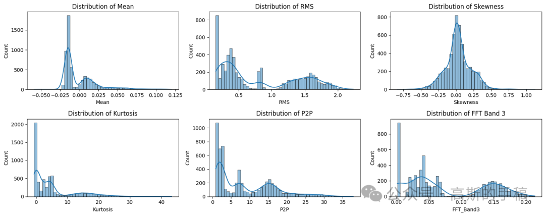
Zhihu Academic Consultation
https://www.zhihu.com/consult/people/792359672131756032
Served as a reviewer for journals such as “Mechanical System and Signal Processing”, “Journal of Electrical Engineering in China”, “Journal of Astronautics”, and “Control and Decision”, with expertise in: signal filtering/noise reduction, machine learning/deep learning, time series pre-analysis/prediction, equipment fault diagnosis/defect detection/anomaly detection