

Click the blue text above to follow us

📋📋📋 The table of contents is as follows: 🎁🎁🎁
Table of Contents
💥1 Overview
📚2 Results
2.1 IEEE 9 Node
2.2 IEEE 68 Node
🎉3 References
🌈4 MATLAB Code, Data, Articles



1 Overview

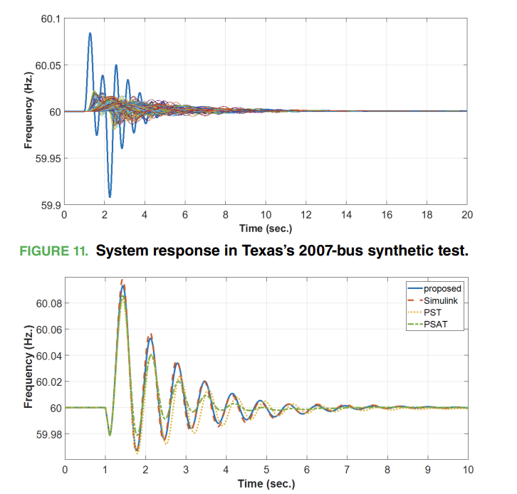
This article introduces a MATLAB-based program developed for dynamic analysis of power systems. It can perform time-domain simulations, system linearization, modal analysis, participation factor analysis and visualization, optimal placement of controllers, selection of feedback signals, frequency response analysis, and control design. In addition to addressing power system issues, the software package also provides symbolic and vectorized representations of models in time domain and state space. The package fully leverages MATLAB’s powerful solvers for solving non-stiff and stiff problems. Both explicit and implicit techniques are used to solve differential algebraic equations (DAE). It is assumed that synchronous machines are equipped with exciters, turbines, and stabilizers. Loads can be modeled as voltage-dependent loads and independent loads. The test systems used in this article are the IEEE 9-node and 68-node systems, as well as the 2007 synthetic power system in Texas. Different types of disturbances are applied to the system, including generator-side and network-side disturbances.


2 Results
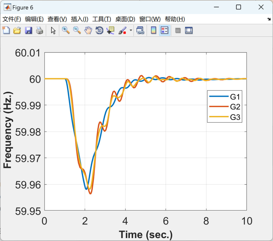
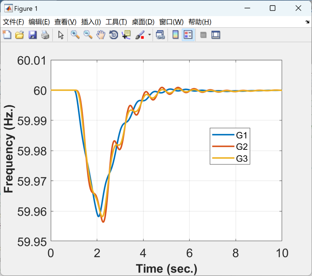
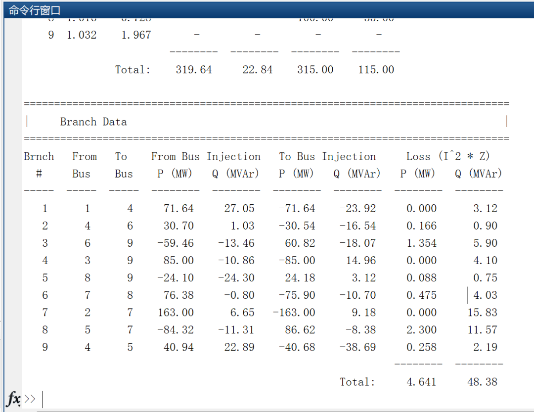
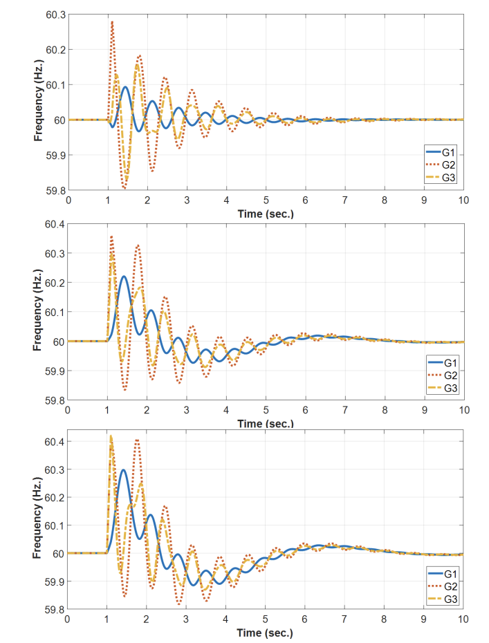
 2.1 IEEE 9 Node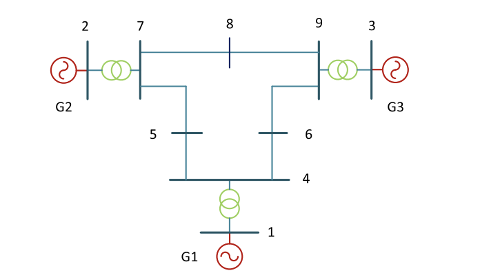
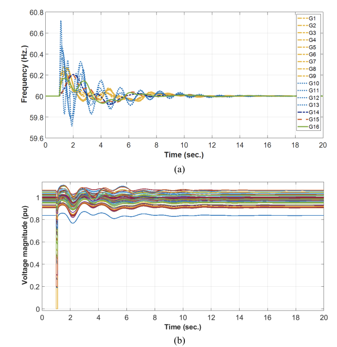
 2.2 IEEE 68 Node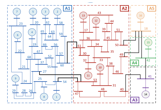
Part of the code:%%%----------------------------% LL-1--------------------------------------T1_LL1 = realp('T1_LL1',1); % T1 coefficient (name and initial value)T2_LL1 = realp('T2_LL1',0.1); % T2 coefficientT1_LL1.Minimum =0.1; T1_LL1.Maximum =1; %Set min-max values for T1T2_LL1.Minimum =0.01; T2_LL1.Maximum =0.1; %Set min-max values for T2T1_LL1.Free =true;T2_LL1.Free =true;LL1=tf([T1_LL1 1],[T2_LL1 1]);%%%----------------------------% LL-2--------------------------------------T3_LL2 = realp('T3_LL2',1); % T3 coefficientT4_LL2 = realp('T4_LL2',0.1); % T4 coefficientT3_LL2.Minimum =0.1; T3_LL2.Maximum =1; %Set min-max values for T3T4_LL2.Minimum =0.01; T4_LL2.Maximum =0.1; %Set min-max values for T4T3_LL2.Free =true;T4_LL2.Free =true;LL2=tf([T3_LL2 1],[T4_LL2 1]);%%%--------------------------Washout---------------------------------------Tw = realp('Tw',1); % Tw coefficientTw.Minimum =1; Tw.Maximum =10;Tw.Free =true;WO=tf([Tw 0],[Tw 1]);%%%--------------------------Gain------------------------------------------Ck = realp('Ck',1); Ck.Minimum =1; Ck.Maximum =50;Kg=tf(Ck);%%%==========================System tuning=================================CL0 = feedback(LL1*LL2*Ck*G,1, -1); % Closed-loop TF (with PSS)CL0.InputName ='ws';CL0.OutputName ='w';Req1 = TuningGoal.Poles(0,0.2,Inf); % [min decay, min damping ratio, max freq].options = systuneOptions('Display','iter');[CL,fSoft] = systune(CL0,Req1, options);sys2=CL.Blocks; OptimizedParam=[sys2.T1_LL1 sys2.T2_LL1 sys2.T3_LL2 sys2.T4_LL2 sys2.Ck]; OptimizedParam=double(OptimizedParam);figure (1) viewGoal(Req1,CL); xlim([-501]); hold on; % Plot the results with the desired goal to check if it is satisfactory%=================================END======================================
3References
Some content in this article is sourced from the internet, and references will be noted. If there are any inaccuracies, please feel free to contact us for removal.



4 MATLAB Code, Data, Articles