Machine Heart Column
This column is produced by Machine Heart SOTA! Model Resource Station and is updated weekly on the Machine Heart WeChat public account every Sunday.
This column will review common tasks in fields such as natural language processing and computer vision, and provide detailed explanations of classic models that have achieved SOTA on these tasks. Go to SOTA! Model Resource Station (sota.jiqizhixin.com) to access the implementation code, pre-trained models, and APIs included in this article.
This article will be serialized in 3 issues, introducing 18 classic models that have achieved SOTA on the machine translation task.
-
Issue 1: RNNsearch, Multi-task, attention-model, Convolutional Encoder, Attention, Value-Network
-
Issue 2: Unsupervised NMT, PBSMT, coarse-to-fine, two-pass decoder translation, XLMs, MASS
-
Issue 3: FlowSeq, mBART, BERT-fused, mRASP, mRASP2, CeMAT
You are reading Issue 1. Go to SOTA! Model Resource Station (sota.jiqizhixin.com) to access the implementation code, pre-trained models, and APIs included in this article.
This Issue’s Model Overview
| Model | SOTA! Model Resource Station Inclusion Status | Model Source Paper |
|---|---|---|
| RNNsearch | https://sota.jiqizhixin.com/project/rnn-search50 Inclusion Count: 6 Supported Frameworks: PyTorch, TensorFlow, etc. | Neural machine translation by jointly learning to align and translate |
| Multi-task | https://sota.jiqizhixin.com/project/multi-task-3 | Multi-task Learning for Multiple Language Translation |
| attention-model | https://sota.jiqizhixin.com/project/attention-model Inclusion Count: 5 Supported Frameworks: PyTorch, TensorFlow, etc. | Effective Approaches to Attention-based Neural Machine Translation |
| Convolutional Encoder | https://sota.jiqizhixin.com/project/convolutional-encoder | A Convolutional Encoder Model for Neural Machine Translation |
| Attention | https://sota.jiqizhixin.com/project/attention-2 Inclusion Count: 5 Supported Frameworks: PyTorch, TensorFlow, etc. | Attention is All You Need |
| Value-Network | https://sota.jiqizhixin.com/project/value-network | Decoding with Value Networks for Neural Machine Translation |
Machine Translation (MT) utilizes the power of machines to “automatically translate text from one natural language (source language) to another (target language).” Machine translation methods can generally be divided into three main categories: Rule-Based Machine Translation (RBMT), Statistical Machine Translation (SMT), and Neural Machine Translation (NMT).
Generally, RBMT analyzes a piece of text by first establishing an intermediate, symbolic representation of the target language. Then, it decides to use either interlingual machine translation or transfer-based machine translation based on the intermediate representation. These methods require sufficient morphological, syntactic, and semantic information, as well as a large number of lexicon rules. A common difficulty with RBMT is the inability to provide adequate and sufficiently large information to satisfy different domains or rules of machine translation.
The primary task of Statistical Machine Translation (SMT) is to construct a reasonable statistical model for language generation, define the model parameters to estimate based on this statistical model, and design parameter estimation algorithms. Early word-based SMT adopted a noise channel model and used maximum likelihood criteria for unsupervised training, while the more recent phrase-based SMT commonly adopts discriminative training methods, generally requiring supervised training with reference corpora.
In 2014, Dzmitry Bahdanau and Yoshua Bengio proposed Neural Machine Translation. NMT, based on deep neural networks, provides an end-to-end solution for machine translation, receiving increasing attention in the research community and gradually being applied in the industry in recent years. NMT models the entire translation process using an RNN-based encoder-decoder framework, where the encoder transforms the source language into a high-dimensional vector through a series of neural network transformations. The decoder is responsible for decoding (translating) this high-dimensional vector back into the target language. During training, it maximizes the likelihood of the target statement given the source statement. During testing, given a source statement x, it seeks a statement y in the target language that maximizes the conditional probability P(y|x). Since the number of possible target statements is exponential, finding the optimal y is NP-hard. Therefore, beam search is typically used to find a reasonable y. Beam search is a heuristic search algorithm that retains the highest scoring partial sequences in a left-to-right manner. Specifically, it maintains a group of candidate partial sequences. At each time step, the algorithm expands each candidate partial statement by adding new words and retains the new candidate statements with the highest scores as rated by the NMT model. The algorithm terminates when the maximum decoding depth is reached or all statements are fully generated (i.e., when all statements contain the EOS symbol suffix).

In this report, we summarize the classic TOP models in Neural Machine Translation.
RNNsearch
RNNsearch is an extension of the encoder-decoder model that learns to jointly align and translate, soft-searching a set of positions in the source sentence that are most relevant to the information set each time a word is generated during translation. The model then predicts the target word based on the context vector associated with these source positions and all previously generated target words. The most important difference between RNNsearch and the basic encoder/decoder is that it does not try to encode the entire input sentence into a single fixed-length vector. Instead, it encodes the input sentence into a series of vectors and adaptively selects a subset of these vectors during the decoding of the translation. This allows the neural translation model to avoid compressing all the information of the source sentence into a fixed-length vector. The RNNsearch architecture includes a (bidirectional RNN) encoder and a decoder, simulating the search of the source sentence during decoding. The conditional probability is as follows:

Unlike the classic encoder-decoder methods, where the probability is conditioned on different context vectors c_i for each target word y_i, the context vector c_i depends on the annotation sequence (h_1, …, h_Tx), where the encoder maps the input sentence into this annotation. Each annotation h_i contains information about the entire input sequence, primarily focusing on the surrounding part of the i-th word in the input sequence. c_i is the weighted sum of these annotations h_i:
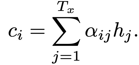
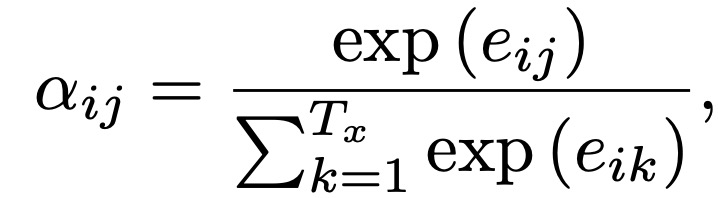
where e_ij is an alignment model that scores the matching degree between the input near position j and the output at position i. The alignment model a is parameterized as a feedforward neural network, which is jointly trained with all other components of the system. Unlike traditional machine translation, the alignment is not treated as a latent variable. Instead, the alignment model directly computes soft alignment, allowing for the gradient of the cost function to be backpropagated. This gradient can be used to jointly train the alignment model along with the entire translation model. The encoder realizes each word’s annotation by summarizing not only the preceding words but also the following words. RNNsearch represents the context as a weighted average of all hidden states of the encoder, where the weights indicate the relevance of each state in the decoder to each state in the encoder. The simple seq2seq model considers that each state in the decoder relates to all information of the input (represented by the last state), while this paper posits that it only relates to relevant states. That is, in the decoder part, the model only focuses on relevant portions and pays little attention to other parts, which resembles human behavior. When a person sees a piece of text or an image, they often focus on a small local area rather than the whole. As shown in Figure 1.
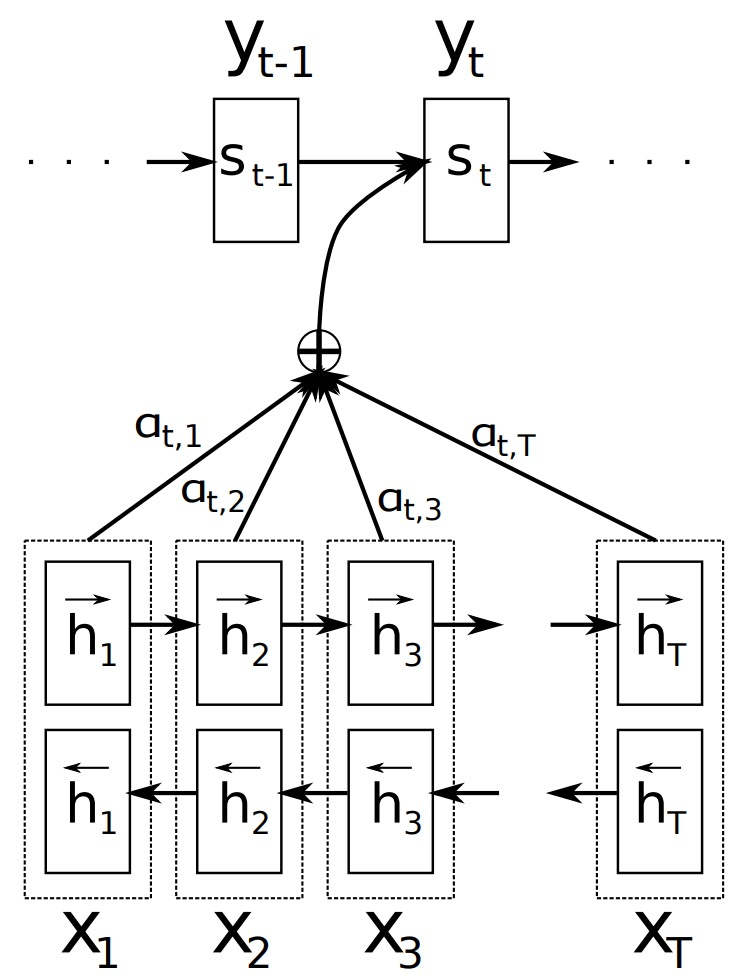 Figure 1. Illustration of the RNNsearch model generating the t-th target word y_t from the given source sentence (x_1, x_2, …, x_T)
The encoder of RNNsearch is a bidirectional RNN (biRNN). A biRNN consists of a forward and a backward RNN. The forward RNN reads the input vectors sequentially and computes the forward hidden state sequence. The backward RNN reads the sequence in reverse order, obtaining a backward hidden state sequence. By linking the forward and backward hidden states, an annotation for each word is obtained. In this way, the annotations can summarize both the preceding and following words. The annotation sequence is used by the decoder and the alignment model to calculate the text vector.
The current SOTA! platform includes 6 model implementation resources for RNNsearch.

| Project | SOTA! Platform Project Detail Page |
|---|---|
RNNsearch |
Go to SOTA! Model Platform to access implementation resources: https://sota.jiqizhixin.com/project/rnn-search50 |
Multi-task
Multi-task is a multi-task learning framework proposed by Baidu to address the issue of data sparsity. In this study, Baidu Translation proposed a multi-task learning neural network translation model with a shared encoder, establishing a unified framework for multilingual translation. As shown in Figure 2.
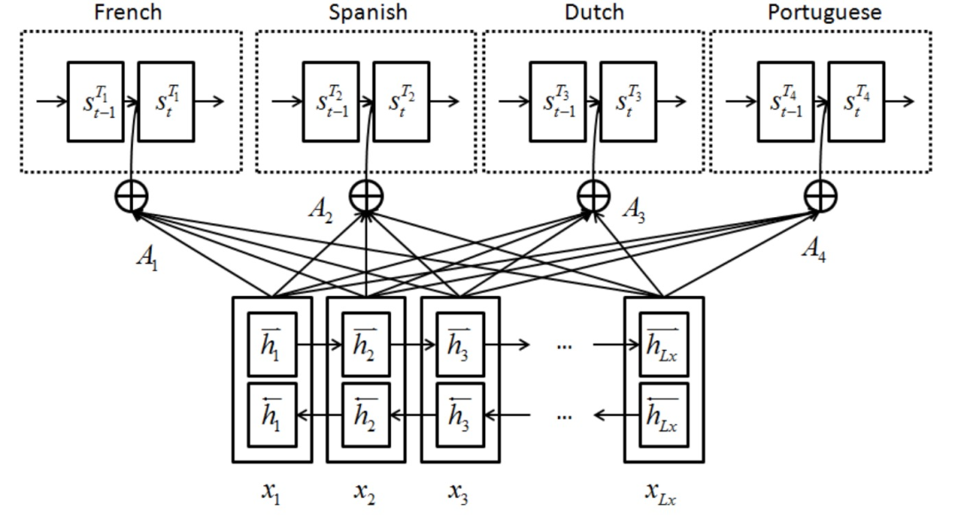 Figure 2. Multi-task learning framework for multi-target language translation
Given a pair of training sentences {x, y}, a standard RNN-based encoder-decoder machine translation model fits a parameterized model to maximize the conditional probability of the target sentence y given the source sentence x, i.e., argmax p(y|x). This can be extended to a multilingual setting. Specifically, suppose we want to translate from English into many different languages, such as French (Fr), Dutch (Nl), and Spanish (Es). Parallel training data is collected beforehand, i.e., En-Fr, En-NL, En-Es parallel sentences. Since the English representations for the three language pairs are shared in one encoder, the optimized objective function is the sum of several conditional probability terms conditioned on the representations produced by the same encoder:

Assuming we have several language pairs. For a specific language pair, given a source sentence input sequence, the goal is to jointly maximize the conditional probability of each generated target word. The probability of generating the t-th target word is estimated as:

g can be seen as a probability predictor with a neural network. (s_t)^Tp is the hidden state of the RNN at time t, which can be estimated as:

The context vector (c_t)^Tp depends on a series of annotations (h_1, …, h_Lx), where the encoder maps the input sentence to these annotations, where Lx is the number of tokens in x. Each annotation h_i is a bidirectional representation, encapsulating the sequence information around the i-th word:
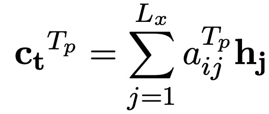
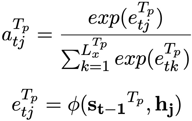
When calculating h_j, a bidirectional RNN is also used.
From a probabilistic perspective, this model can learn the conditional distributions of several target languages in the same source corpus. Therefore, the RNN encoder-decoder is jointly trained by summing several conditional probabilities. As for the bidirectional RNN module, a gated recurrent neural network is used. In the multi-task learning framework, the parameters of the gated recurrent neural network in the encoder are shared, expressed as:

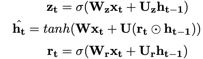
The recursive computation process is illustrated in Figure 3, where x_t represents the one-hot vector of the t-th word in the sequence.
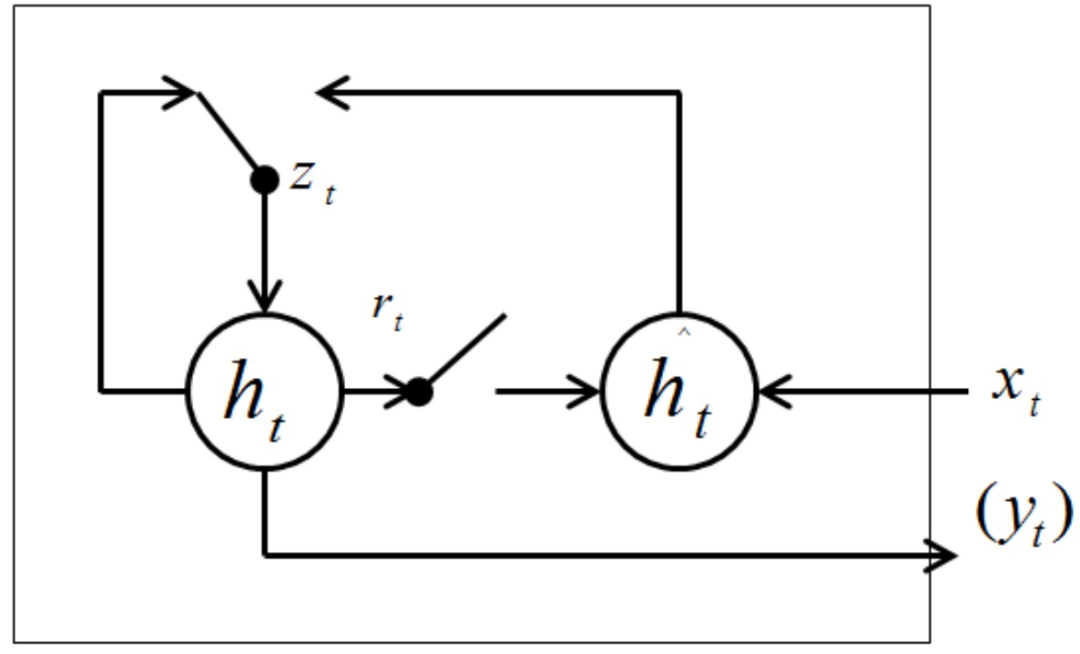 Figure 3. Gated recurrent neural network computation, where r_t is the reset gate responsible for eliminating memory cells, and z_t can be regarded as the soft weight between current state information and historical information.
| Project | SOTA! Platform Project Detail Page |
|---|---|
Multi-task |
Go to SOTA! Model Platform to access implementation resources: https://sota.jiqizhixin.com/project/multi-task-3 |
attention-model
This paper mainly proposes Global attention and Local attention, that is, two types of attention mechanisms: a global method that always focuses on all source words and a local method that only looks at a subset of source words at a time. The commonality of these two types of models is that in each time step t during the decoding phase, both methods first take the hidden state h_t at the top layer of the stacked LSTM as input. The goal is to obtain a context vector c_t that captures relevant source-side information to help predict the current target word y_t. Although these models differ in how they obtain the context vector c_t, they share the same subsequent steps.
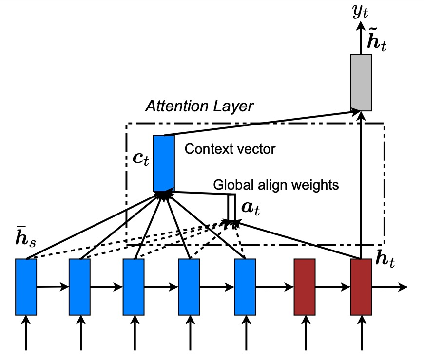
Figure 4: Global attention model—at each time step t, this model derives a variable-length alignment weight vector a_t based on the current target state h_t and all source states h¯s. Then, a global context vector c_t is calculated based on a_t, which is the weighted average of all source states
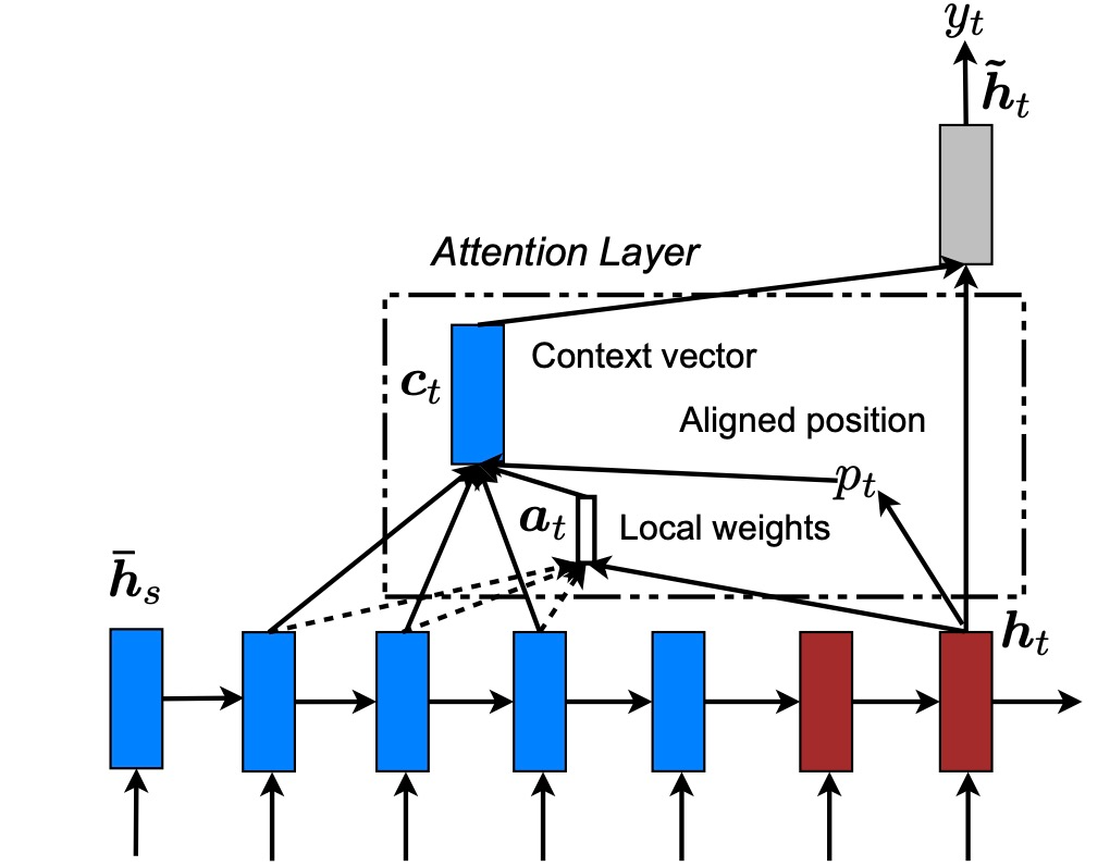
Figure 5: Local attention model—this model first predicts a single alignment position p_t for the current target word. Then, it calculates the context vector c_t as the weighted average of the source hidden states within a window centered on the source position p_t. The weights are inferred from the current target state h_t and the source states h¯s within the window
Given the target hidden state h_t and the source-side context vector c_t, a simple concatenation layer is used to combine the information from these two vectors, generating an attention hidden state as follows:

The attention vector h˜t is fed back through a softmax layer to generate a prediction distribution, expressed as:
Global attention. The idea of the global attention model is to consider all hidden states of the encoder when deriving the context vector c_t. In this type of model, by comparing the current target hidden state h_t with each source hidden state h¯s, a variable-length alignment vector a_t is obtained, whose size equals the number of time steps on the source side:
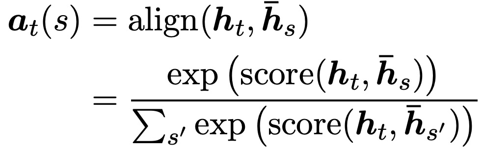
Here, the score is called a content-based function, considering three different choices:
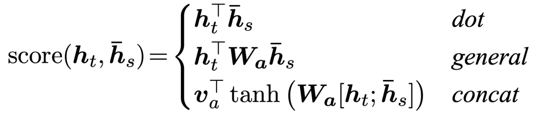
Additionally, a position-based function is used, where the alignment score is calculated solely from the target hidden state h_t, as follows:

Considering the alignment vector as weights, the context vector c_t is calculated as the weighted average of all source hidden states. Local attention. The global attention has a disadvantage that it must focus on all words in the source for each target word, which can be impractical when translating longer sequences, such as paragraphs or documents. To address this drawback, a local attention mechanism is proposed, which selectively focuses on a small number of source positions for each target word. The local attention mechanism concentrates on a small background window and is differentiable. This method’s advantage is that it avoids the expensive computational cost required in soft attention while being easier to train than hard attention methods. Specifically, this model first generates an alignment position p_t for each target word at time t. Then, it derives the context vector c_t as the weighted average of the set of source hidden states within the window [pt-D, pt+D]; D is chosen empirically. Unlike the global method, the current local alignment vector a_t has a fixed dimension, i.e., ∈R^2D+1. Considering the following two variants of the model: Monotonic alignment (local-m) — simply set p_t = t, assuming the source and target are largely monotonically aligned. Predictable alignment (local-p) — the model no longer assumes monotonic alignment but predicts an alignment position as follows:

W_p and v_p are parameters of the model used to learn to predict positions. S is the length of the source sentence. The result of the sigmoid ensures that p_t ∈ [0,S]. To bring the alignment point closer to p_t, a Gaussian distribution centered on p_t is placed. Specifically, the alignment weights are defined as:

Input-feeding method. In both global and local methods, the attention decisions are made independently. In standard machine translation, it is common to maintain a coverage set during translation to track which source words have been translated. Similarly, in attention NMT, past alignment information should be considered when making decisions. To address this issue, an input-feeding method is proposed, where the attention vector h_t is concatenated with the input at the next time step, as shown in Figure 6. This concatenation has two effects: (a) it hopes to make the model more comprehensively focus on previous alignment choices; (b) it creates a very deep network that expands both horizontally and vertically.
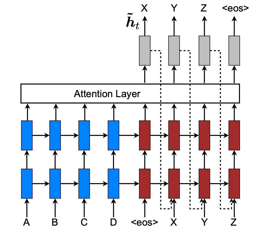 Figure 6. input-feeding—inputting the attention vector h˜t into the next time step to inform the model of past alignment decisions.
The current SOTA! platform includes 5 model implementation resources for the attention model.

| Project | SOTA! Platform Project Detail Page |
|---|---|
| attention-model | Go to SOTA! Model Platform to access implementation resources: https://sota.jiqizhixin.com/project/attention-model |
Convolutional Encoder
Convolutional Encoder is a model based on convolutional layers, which allows for simultaneous encoding, unlike recurrent neural networks that are constrained by temporal dependencies. A simple benchmark for non-recurrent encoders is the pooling model mentioned by Ranzato, which averages the embeddings of K consecutive words. Besides the proximity of words in the input, averaging word embeddings does not express positional information. Therefore, positional embeddings are introduced to encode the absolute position of each word in the sentence. Thus, each embedding e_j in the source sentence contains a positional embedding l_j and a word embedding w_j. Similar to the recurrent encoder, the attention scores a_ij are computed from the pooled representation z_j, and the conditional input c_i is the weighted sum of the embeddings e_j:
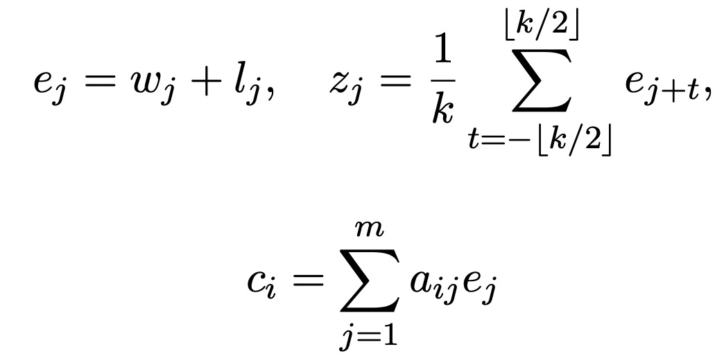
A direct extension of pooling is to learn kernels in convolutional neural networks (CNNs). The output z_j of the encoder contains fixed-size contextual information depending on the kernel width k, but the required context width may vary. This can be addressed by stacking several layers of convolution and non-linearity: additional layers increase the total contextual size, while non-linearity can adjust the effective size of the context as needed. For example, stacking 5 convolutions with a kernel width of k=3 will yield an input domain of 11 words, meaning each output depends on 11 input words, and non-linearity allows the encoder to utilize the entire input domain or focus on fewer words as needed. To facilitate the learning of deep encoders, residual connections of each convolution’s input are added to the output, followed by applying a non-linear activation function to the output. Multi-layer CNNs are constructed by stacking several blocks together. CNNs do not include pooling layers typically used for downsampling, meaning that the full source sequence length is retained after the application of the network. Similar to the pooling model, the convolutional encoder uses positional embedding methods. The final encoder consists of two stacked convolutional networks (Figure 7). CNN-a generates encoder output z_j to compute attention scores a_i, while the conditional input c_i of the decoder is computed by summing the outputs of CNN-c:

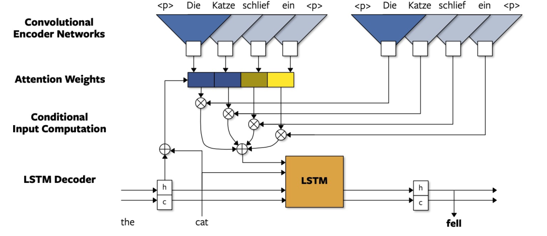
Figure 7. Neural machine translation model with a single-layer convolutional encoder network. CNN-a on the left, CNN-c on the right. The embedding layer is not shown.
The current SOTA! platform includes Convolutional Encoder with a total of 1 model implementation resource.

| Project | SOTA! Platform Project Detail Page |
|---|---|
| Convolutional Encoder | Go to SOTA! Model Platform to access implementation resources: https://sota.jiqizhixin.com/project/convolutional-encoder |
Attention
In 2017, the Google Translation team published “Attention is All You Need,” completely discarding network structures such as RNNs and CNNs, and solely using the Attention mechanism to complete machine translation tasks, achieving excellent results. The attention mechanism has also become a research hotspot. Most competitive neural sequence transduction models have an encoder-decoder structure. The encoder maps the input symbol representation sequence (x1, …, xn) to a sequence of continuous representations z=(z1, …, zn). Given z, the decoder generates a sequence of output symbols (y1, …, ym) one element at a time. At each step, the model is autoregressive, using previously generated symbols as additional input when generating the next symbol. The Transformer follows this overall architecture, employing stacked self-attention and point-wise fully connected layers in both the encoder and decoder, as shown in the left and right parts of Figure 8.
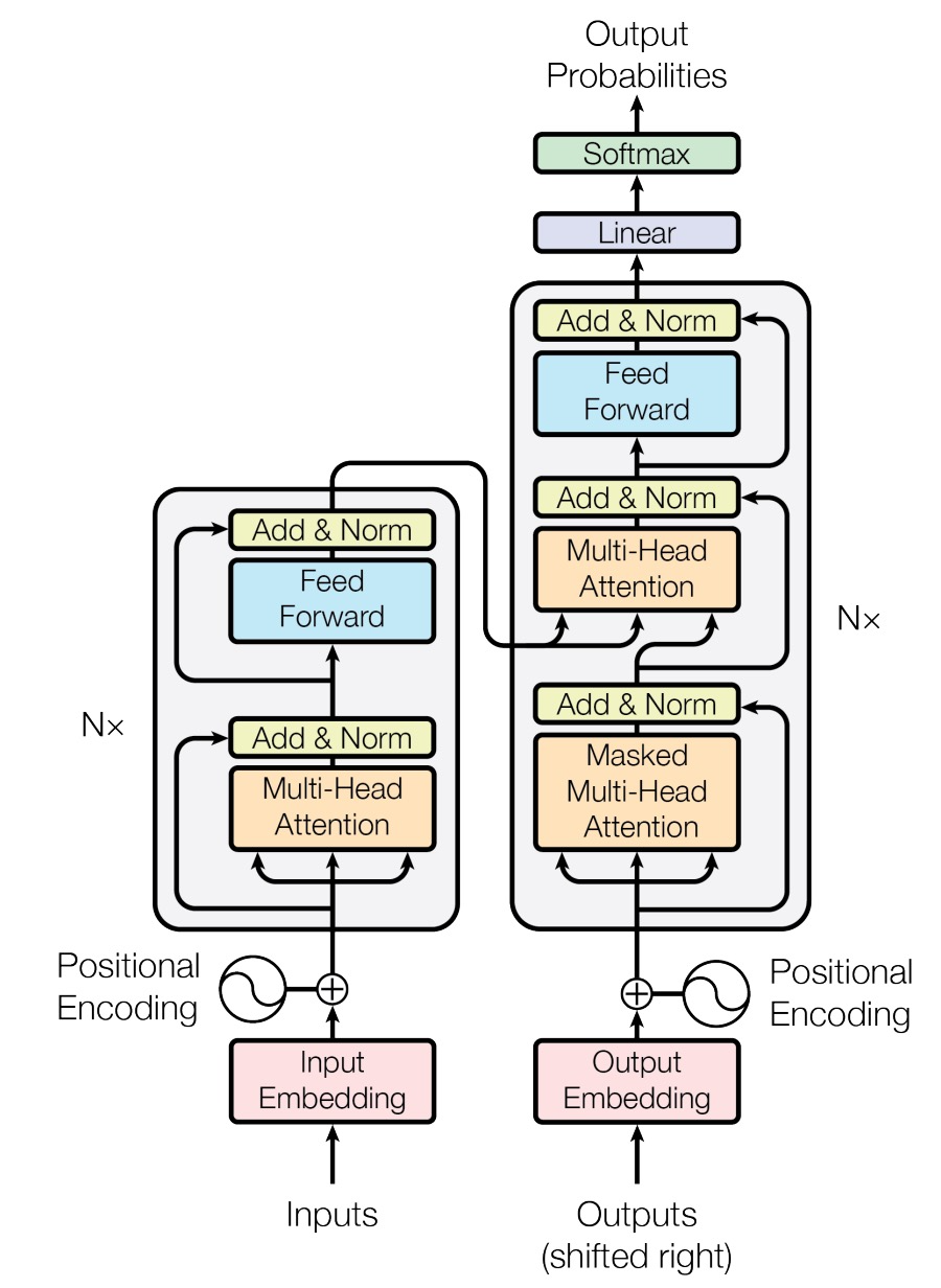 Figure 8. Transformer architecture
Encoder
The encoder is composed of N=6 identical layers stacked on top of each other. Each layer has two sub-layers. The first layer is a multi-head self-attention mechanism, and the second layer is a simple, position-wise fully connected feedforward network. A residual connection is applied around each of the two sub-layers, followed by layer normalization. That is, the output of each sub-layer is LayerNorm(x + Sublayer(x)), where Sublayer(x) is the function implemented by the sub-layer itself. To facilitate these residual connections, all sub-layers in the model, as well as the embedding layer, generate outputs of size dmodel=512. Decoder
The decoder is also composed of a stack of N=6 identical layers. In addition to the two sub-layers of each encoder layer, the decoder also inserts a third sub-layer that performs multi-head attention over the output of the encoder stack. Similar to the encoder, a residual connection is applied around each sub-layer, followed by layer normalization. The self-attention sub-layer in the decoder stack is further modified to prevent positions from attending to subsequent positions. This masking, combined with the fact that the output embedding is offset by one position, ensures that predictions for position i depend only on known outputs at positions less than i. Attention. The attention function can be described as mapping a query and a set of key-value pairs to an output, where the query, keys, values, and output are all vectors. The output is computed as a weighted sum of the values, where the weights assigned to each value are computed by a compatibility function of the query with the corresponding key. The attention used in the Transformer is Scaled Dot-Product Attention, which is normalized dot-product attention. Assuming the input query q and key dimensions are dk, and value dimensions are dv, the dot product operation is computed between the query and each key, divided by dk, and then the softmax function is applied to compute the weights. A schematic of Scaled Dot-Product Attention is shown in Figure 9 (left).
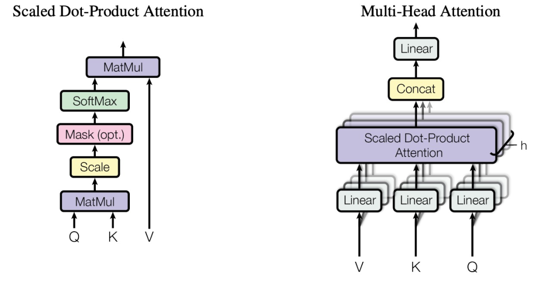
Figure 9. (Left) Scaled Dot-Product Attention. (Right) Multi-head attention consists of several attention layers running in parallel.
If it is not enough to perform such weight operations on Q, K, and V just once, Multi-Head Attention is proposed, as shown in Figure 9 (right). The specific operations include:
-
First, perform a linear mapping on Q, K, and V, mapping the input dimensions of Q, K, V matrices, all of size dmodel, to Q∈Rm×dk, K∈Rm×dk, V∈Rm×dv;
-
Then, use Scaled Dot-Product Attention to compute the result;
-
Repeat the above two steps multiple times, then merge the obtained results;
-
Perform a linear transformation on the merged result.
In the architecture of Figure 8, there are three Multi-head Attention modules, which are:
-
Self-Attention in the Encoder module, where the input Q=K=V for each layer is the output of the previous layer. Each position in the Encoder can access the output of all positions from the previous layer.
-
Mask Self-Attention in the Decoder module, where each position can only access information from previous positions, thus requiring masking, set to -∞.
-
Attention between Encoder and Decoder, where Q comes from the output of the previous Decoder layer, and K, V come from the output of the encoder, allowing each position in the decoder to access all position information of the input sequence.
After performing the Attention operation, each layer in the encoder and decoder contains a fully connected feedforward network that performs the same operation on the vector for each position, including two linear transformations and a ReLU activation output:

Because the model does not include recurrence/convolution, it cannot capture sequential order information. For example, if K and V are shuffled row-wise, the result after Attention remains the same. However, sequential information is crucial as it represents the global structure, hence the relative or absolute positional information of the sequence must be utilized. Here, the position embedding vector dimension for each token is also dmodel=512, and then the original input embedding and position embedding are added together to form the final embedding as the input to the encoder/decoder. The position embedding calculation formula is as follows:

where pos represents position, and i represents dimension. That is, each dimension of the position encoding corresponds to a sine wave. The wavelength forms a geometric series from 2π to 10000-2π. This function is chosen because it allows the model to easily learn to participate based on relative positions, as for any fixed offset k, PE_pos+k can be represented as a linear function of PE_pos.
The current SOTA! platform includes Attention a total of 4 model implementation resources.

| Project | SOTA! Platform Project Detail Page |
|---|---|
| Attention | Go to SOTA! Model Platform to access implementation resources: https://sota.jiqizhixin.com/project/attention-2 |
Value-network
The idea of the Value-network is to use a predictive network to improve beam search. The source sentence x, the currently available decoding outputs y1,…, yt-1, and the candidate words w at step t are used as inputs to predict the long-term value of the partial target sentence (e.g., BLEU score). Following the conventions of reinforcement learning, this predictive network is called the value network (Value-network). Specifically, a recurrent structure is proposed for the value network, and its parameters are trained using bilingual data. During testing, when selecting a word w for decoding, both the conditional probability given by the NMT model and the long-term value predicted by the value network are considered. In traditional reinforcement learning, the value function describes how much cumulative reward can be obtained from state s by following some policy π. In machine translation, any input sentence x paired with the partial output sentence y_ can be viewed as a state, and the translation model π_Θ can be viewed as a policy that can generate a word (action) in any state. Given the policy π_Θ, the value function characterizes what the expected translation performance (e.g., BLEU score) would be if π_Θ is used to translate x, with the first t-1 words being y_. Let v(x, y_) represent the value function, and y^∗(x) represent the ground-truth translation, then:

where Y is the space of the complete sentence. The first important question is how to design the input and the parameterized form of the value function. Since the translation model is built on the encoder-decoder framework, we also establish the value network on this architecture. To fully utilize the information in the encoder-decoder framework, a value network with two new modules is developed, namely the semantic matching module and the context coverage module.
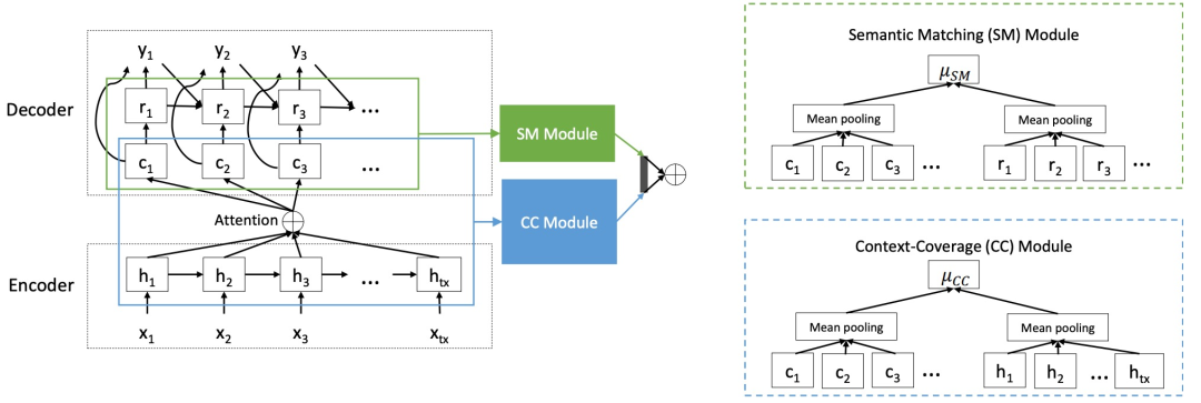 Figure 10. Value-network architecture
The Semantic Matching (SM) module. In the semantic matching module, at time step t, mean pooling is applied to the hidden state of the decoder RNN:

as a summary sentence of the partial target sentence. Additionally, the average set method of the context state is used:
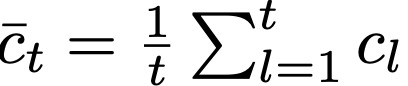
as a context summary in the source language. By concatenating r¯t and c¯t, and using a feedforward network as follows to evaluate the semantic information between the source sentence and the target sentence:

The Context-Coverage (CC) module. It has been observed that the more context covered in the attention model, the better the translation results. Therefore, a context coverage module is constructed to measure the information coverage used in the encoder-decoder framework. Applying mean pooling on the context layer and encoding state can provide some effective knowledge. Let:
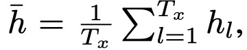
We use another feedforward network to process this information:

Finally, µSM and µCC are concatenated, and another fully connected layer with a sigmoid activation function is used to output a scalar as the predicted value. The entire architecture is illustrated in Figure 10.

| Project | SOTA! Platform Project Detail Page |
|---|---|
| Value-Network | Go to SOTA! Model Platform to access implementation resources: https://sota.jiqizhixin.com/project/value-network |
Go to SOTA! Model Resource Station (sota.jiqizhixin.com) to access the implementation code, pre-trained models, and APIs included in this article.
Web access: Enter the new site address sota.jiqizhixin.com in the browser address bar to go to the “SOTA! Model” platform to check if new resources have been added for the models you are interested in.
Mobile access: Search for the service account name “Machine Heart SOTA Model” or ID “sotaai” in the WeChat mobile app, follow the SOTA! Model service account, and use the platform features through the bottom menu bar of the service account. You will also receive regular updates on the latest AI technologies, development resources, and community dynamics.