In wireless communication systems, certain application scenarios may require changing the bandwidth of filters. Recently, my project had a requirement for an online change of filter bandwidth. So how can we implement the online switching of filter bandwidth? In fact, Xilinx’s FIR Compiler IP has this capability. Let’s follow along to see how to set it up.
1. Implementation Overview
Xilinx’s FIR Compiler IP provides two methods for changing bandwidth, as follows:
(1) Reload Mode
Using the IP’s reload interface, you can write any set of filter coefficients you want to configure. However, the reload interface is a 16-bit wide AXI-Stream interface, which requires some interface conversion when interfacing with software, making it slightly more complex to implement.
(2) Config Mode
You need to prepare multiple sets of filter coefficients in advance, with the same order of coefficients for each set. Then, these coefficients are combined into a single group and filled into the Coefficient Vector or Coefficient File. By writing the index of each set of filter coefficients through the config interface, you can load the corresponding set of filter coefficients. Compared to the reload mode, the advantage of the config mode is that it is simpler to implement; you only need to control the switching signal online. The downside is that it lacks flexibility, as you can only switch between the pre-prepared sets of filter coefficients and cannot truly configure arbitrary filter coefficients.
This article will focus on the implementation of the config mode, as applications that can be quickly developed are good applications.
2. Generation of Filter Coefficients
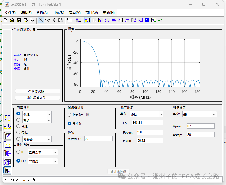
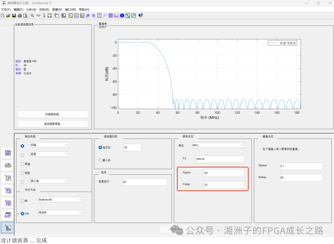
I used Matlab to generate the required filter coefficients. In the following figure, I designed two different low-pass filters, where the first filter has a passband of 3.6M and a cutoff frequency of 30.72M; the second filter has a passband of 30M and a cutoff frequency of 55M.
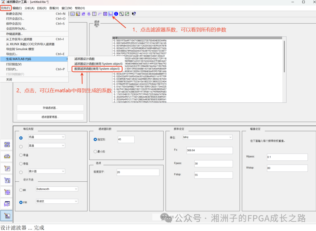
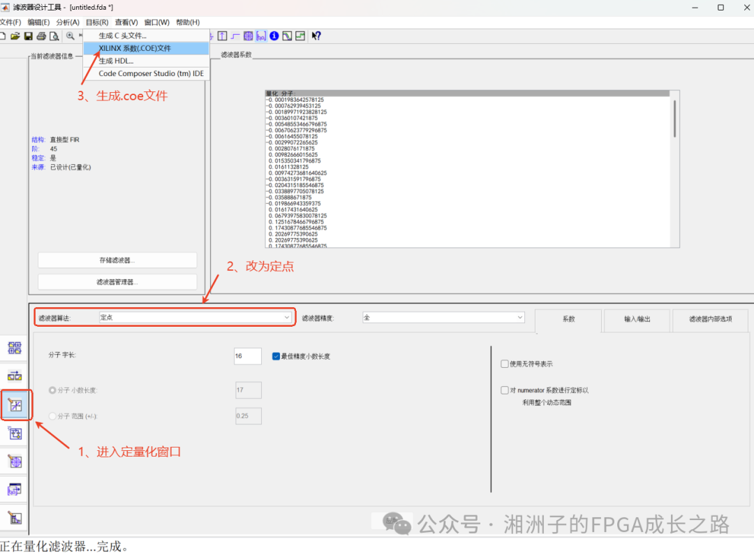
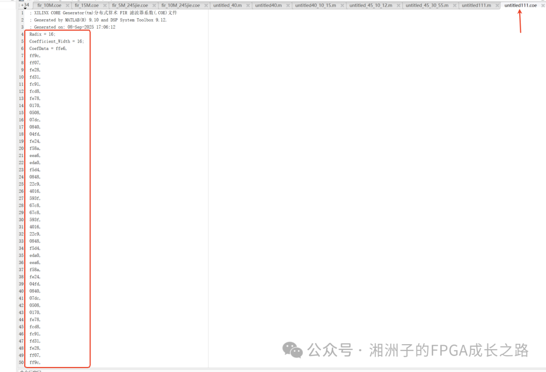
Then we export the filter coefficients from Matlab. There are also two methods for this, and I will demonstrate both methods using the export of the 30M filter coefficients as an example.
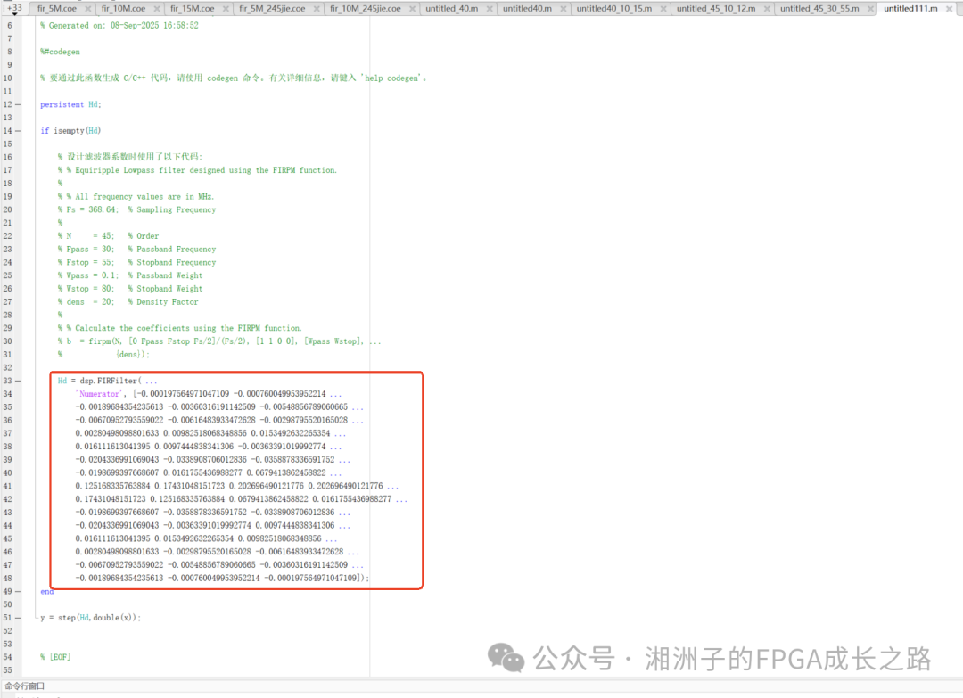
(1) Vector Method
(2) COE File Method
3. Configuration of FIR Compiler IP in Config Mode
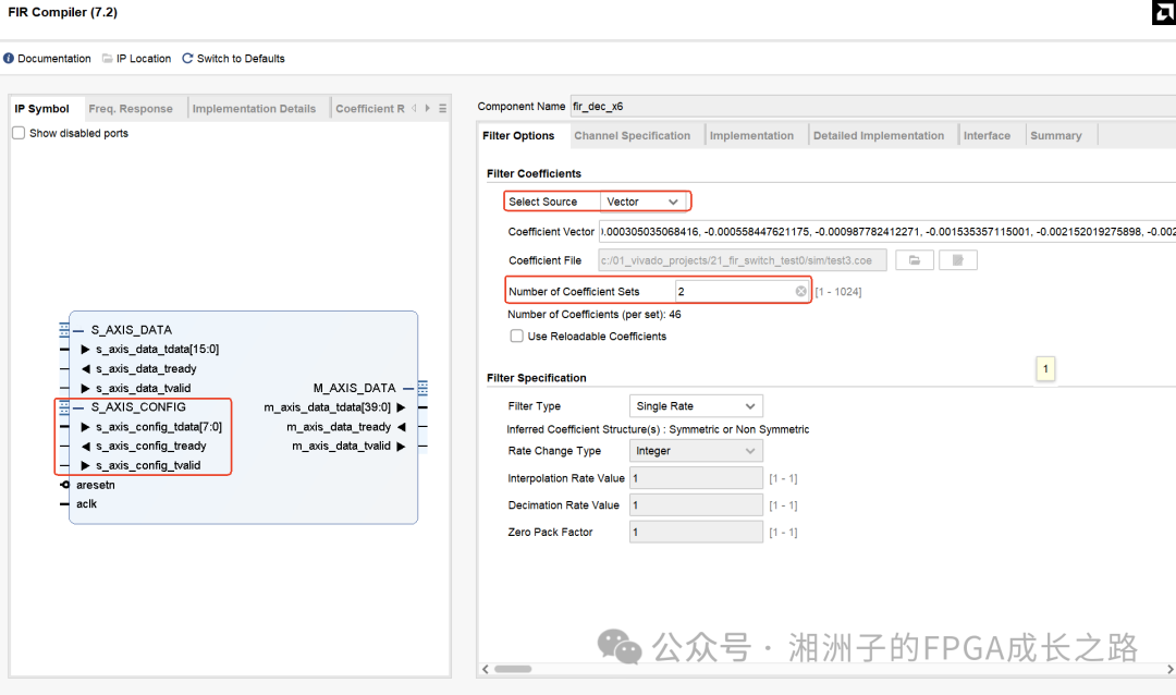
I used the vector method to import filter coefficients into the IP. Since I used two sets of filter coefficients, the Number of Coefficient Sets was set to 2. We can also see that the IP now has an additional S_AXIS_CONFIG interface.
So how do we fill multiple sets of filter coefficients into the IP? There are also two methods for this—vector and coe. Below, I provide examples for both.
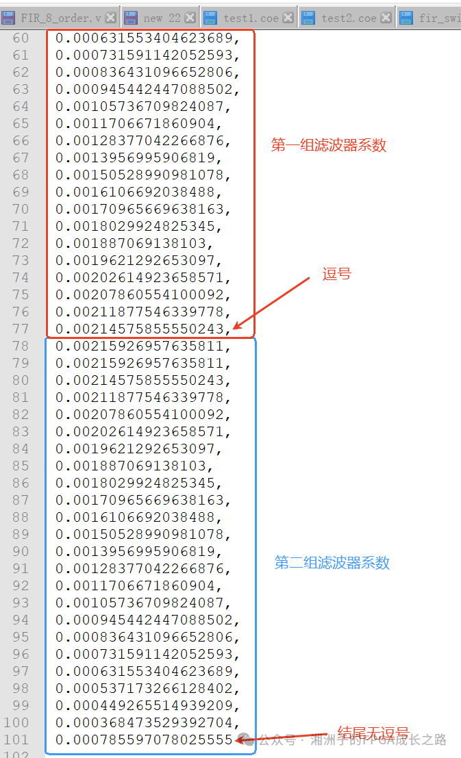
(1) Vector Method
Concatenate the two sets of coefficients of the same order in sequence, separating them with commas, and no comma is needed at the end, as shown in the figure below:
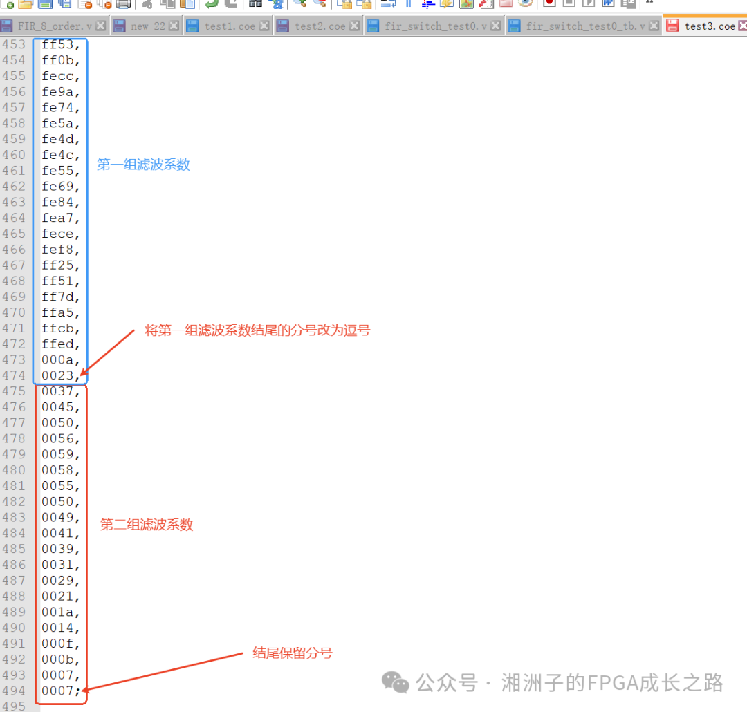
(2) COE File Method
The filter coefficients in the COE file are in hexadecimal format. Similarly, concatenate the two sets of filter coefficients in sequence, changing the semicolon at the end of the first set of coefficients to a comma, and keep the semicolon at the end of the last coefficient.
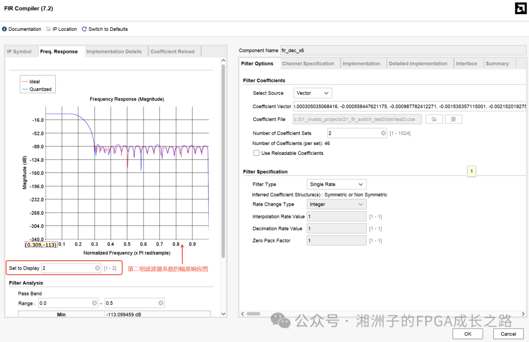
 After filling the two sets of filter coefficients into the IP, we can click on the IP’s Freq Response interface to view the amplitude response of each set of filter coefficients, as shown in the figure below: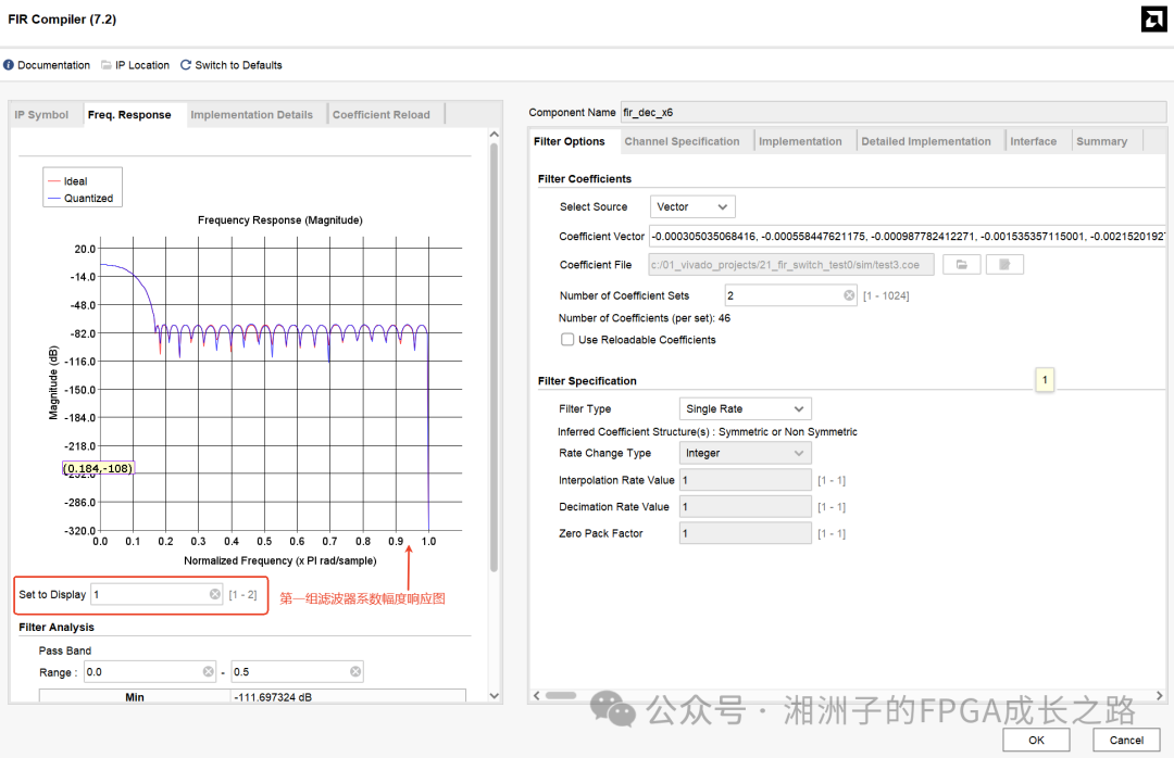
4. Configuration Principle of Config Interface
The signal composition of the config interface is shown in the figure below:
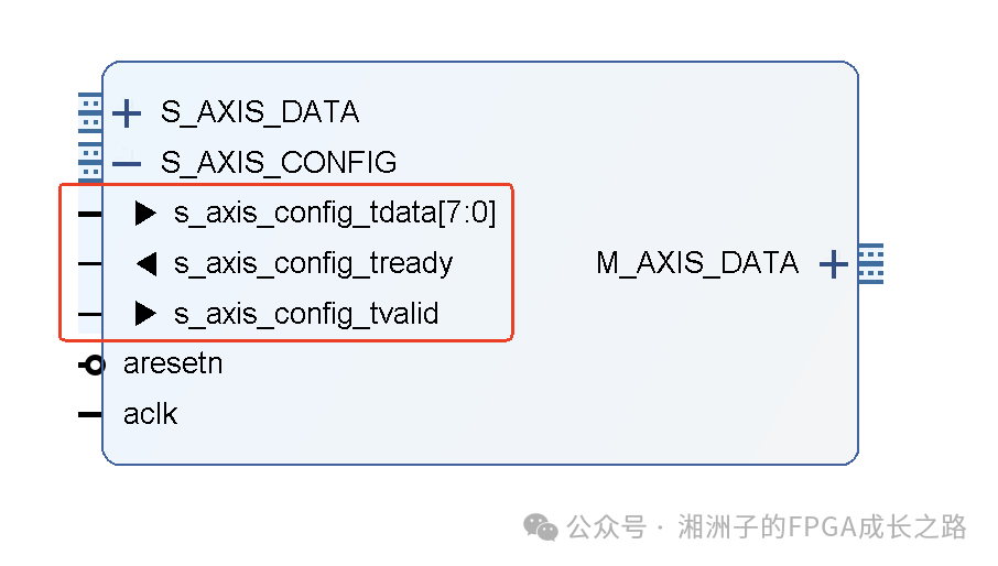
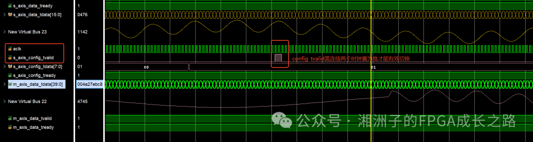
When switching filter coefficients using the config mode, you only need to control the s_axis_config_tvalid and s_axis_config_tdata signals. I consulted the PG149 manual, which did not provide specific usage. Subsequently, I simulated and tried several times to understand their meanings and working principles, as follows:
|
Signal Name |
Meaning |
|
s_axis_config_tdata |
The index of the filter coefficient set; writing 0 corresponds to the first set, writing 1 corresponds to the second set, and so on. |
|
s_axis_config_tvalid |
The valid signal for config_tdata, which must be high for two consecutive clock cycles to be valid. |
|
s_axis_config_tready |
When high, it indicates that the IP can receive data, and data can only be written at this time. |
5. Simulation Testing
5.1. Testing Approach
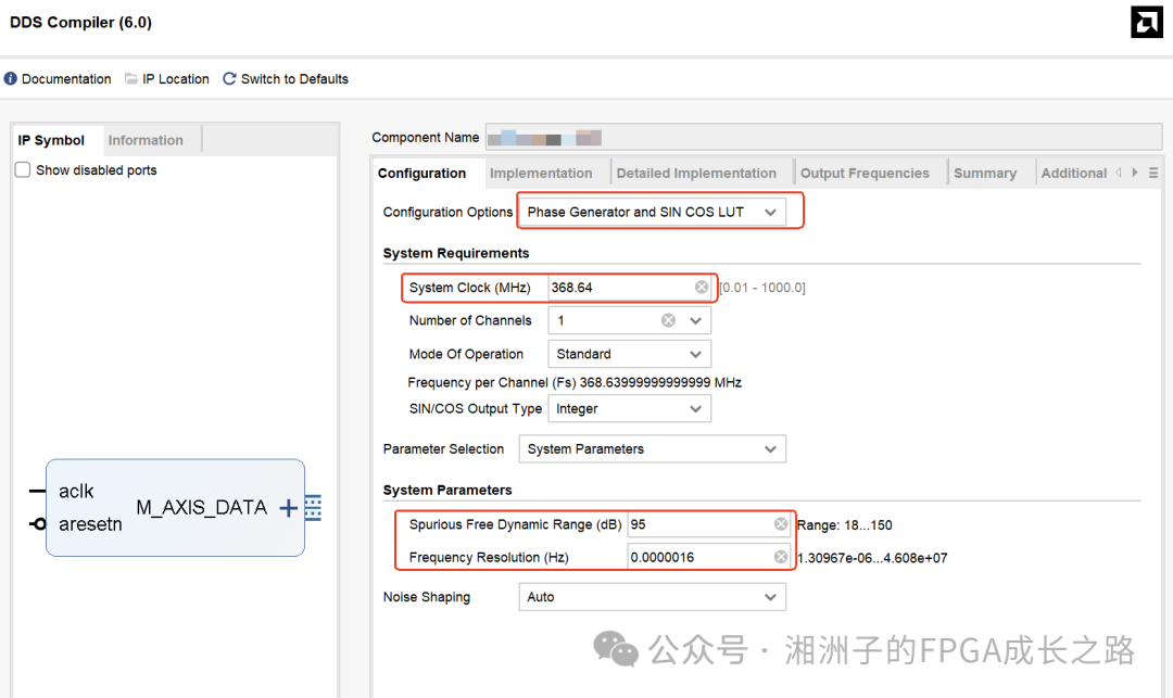
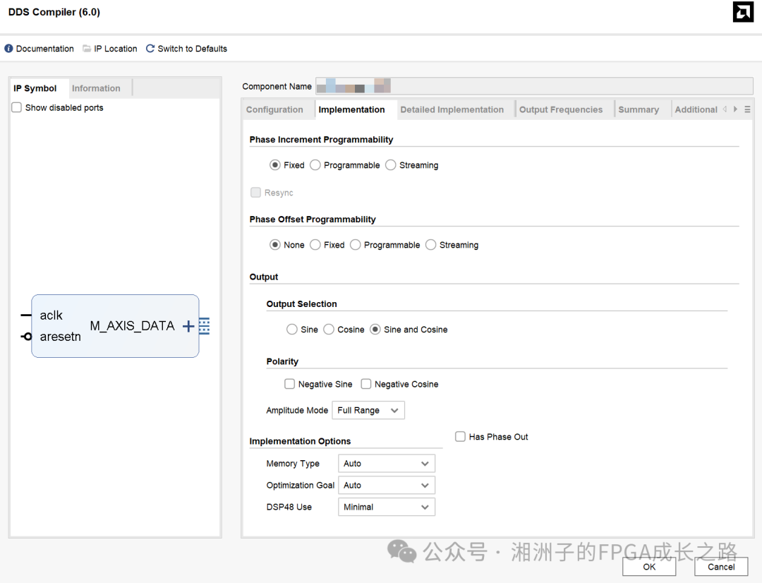
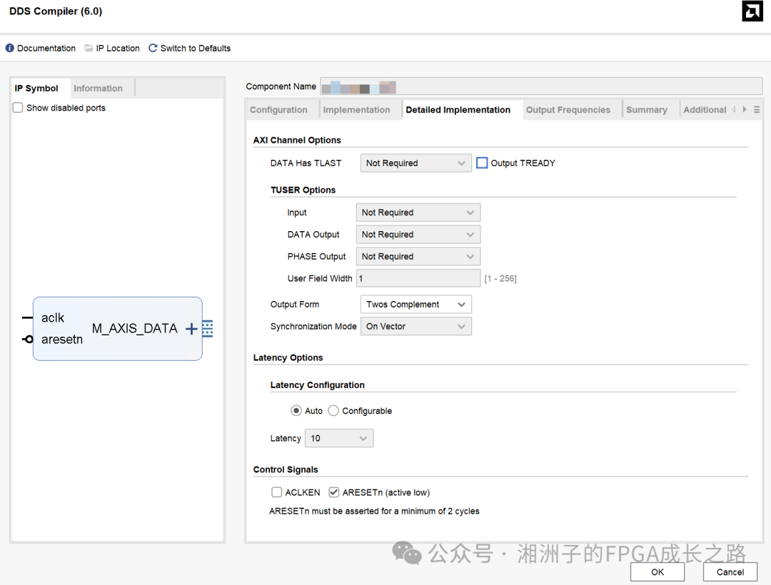
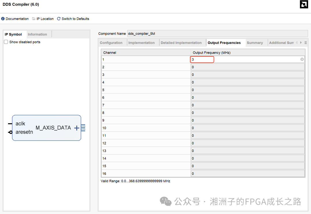
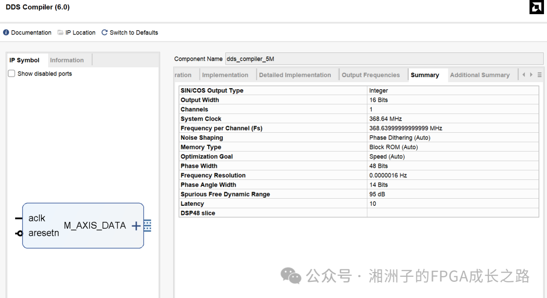
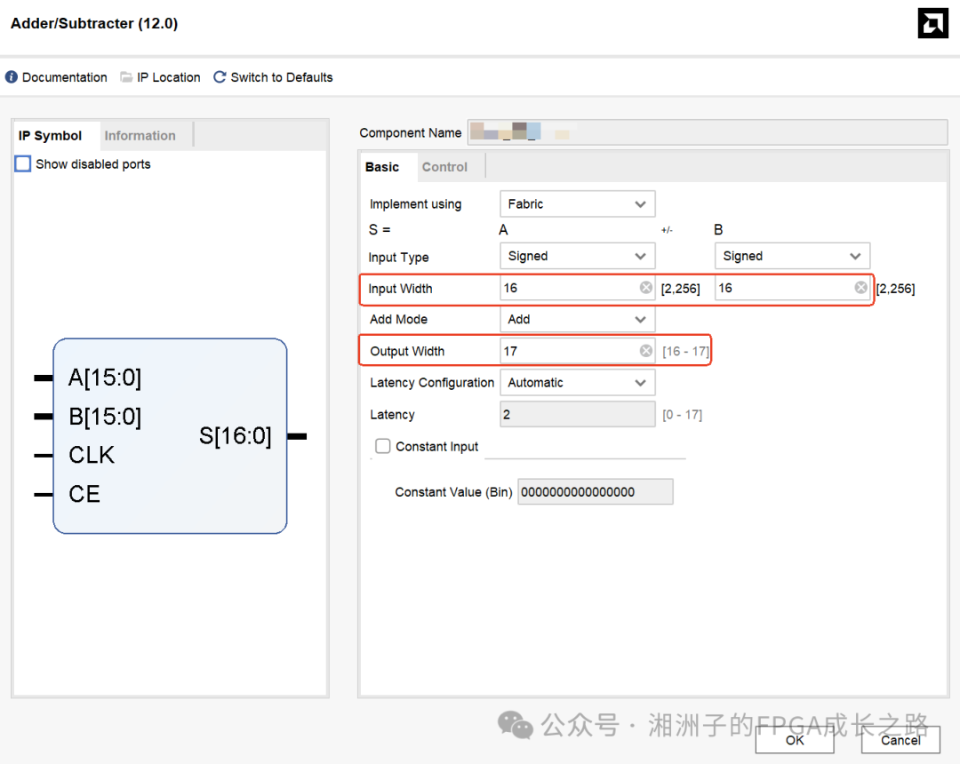
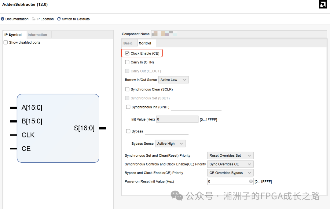
I used two DDS Compiler IPs as signal sources. DDS0 generates a sine wave with a bandwidth of 3M, and DDS1 generates a sine wave with a bandwidth of 30M. Then, I used an Adder to mix these two sine waves and send them into the FIR filter. Finally, I configured the config interface to switch the filter coefficients and observed the waveform output of the filter to see if the switching effect was achieved. Below are the specific configurations for the DDS IP and Adder IP.
(1) DDS Configuration:
(2) Adder Configuration:
5.2. Control Logic Code
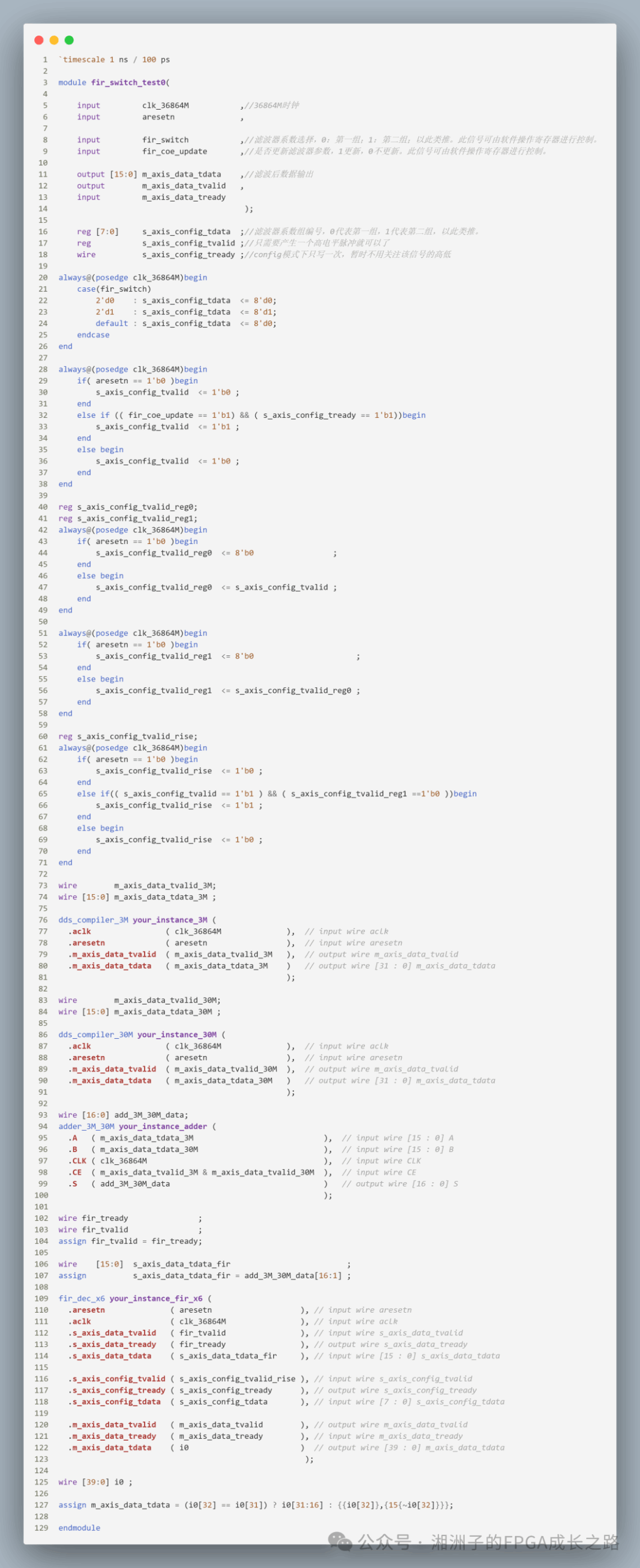
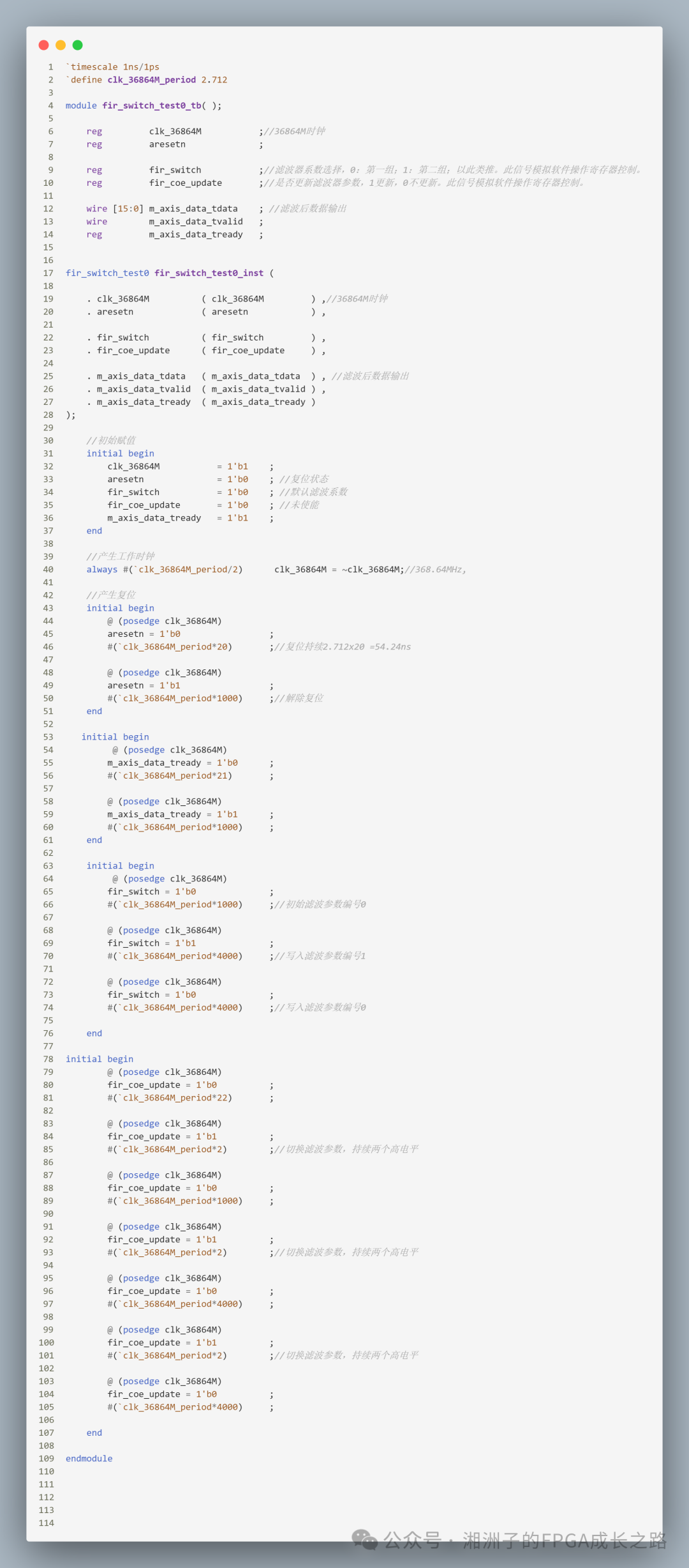
There are two points to note in the control logic code: first, the valid config_tvalid signal must maintain a high level for 2 clock cycles; I generated this signal using a clocking method. Second, the output data of the FIR filter must undergo saturation processing to prevent data overflow; readers can search online for more information on this. My specific code is as follows:
5.3. Simulation Code
The simulation code is written quite clumsily, haha, readers can just take a look 


 !
!
5.4. Simulation Test Results
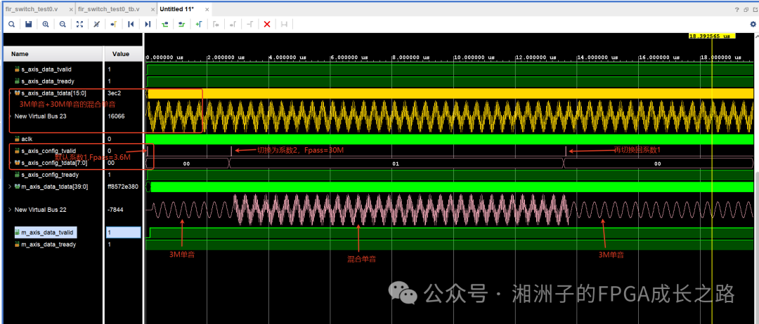
From the above figures, it can be seen that when using the first set of filter coefficients, the 30M bandwidth sine wave can be filtered out, so the output only has a 3M bandwidth sine wave. After switching to the second set of filter coefficients in config mode, both the 3M sine wave and the 30M sine wave can be output, thus achieving the dynamic switching of filter coefficients.
Additionally, let’s take a closer look at how long it takes for the filter to take effect after switching filter coefficients.
I checked the first filter coefficient switch, as shown in the figure below. After setting the coefficient switch, the new filter coefficients take effect after 31 clock cycles.
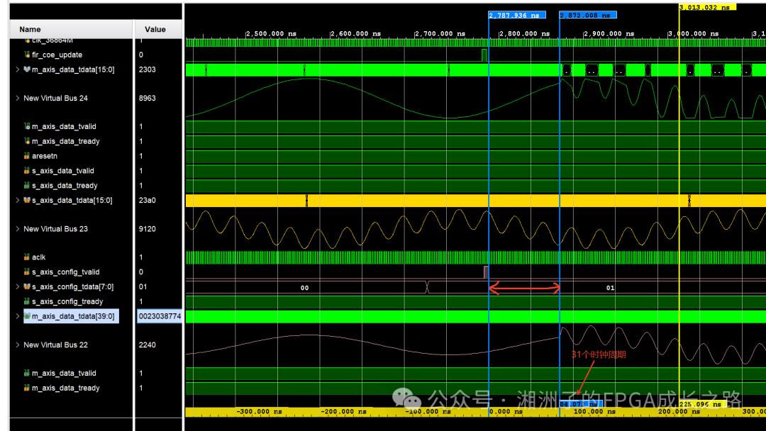
I checked the second coefficient switch, as shown in the figure below. After setting the coefficient switch, the new filter coefficients take effect after 32 clock cycles.
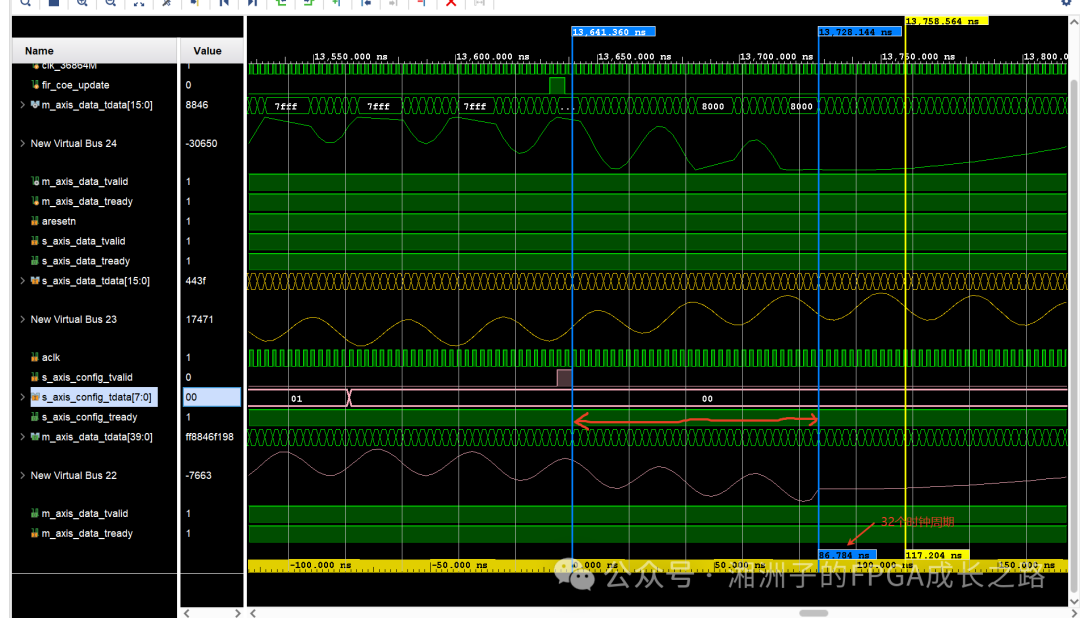
Here, I am a bit curious as to why the effective time after switching filter coefficients is not strictly the same for both switches. If anyone has insights, please share. However, the effective time difference between the two coefficient switches is not significant. In the future, if software controls the config interface and requires frequent switching of filter coefficients, this timing may need to be noted.