“ Sharing basic operations of Geopandas.”
First, here is the link to the sample data:
https://pan.baidu.com/s/1bAnUo0S_ojxXdkyBqWAnLg?pwd=gxu2 Extraction code: gxu2
01
—
Reading and Saving Shapefiles
Using the gpd.from_file() function from geopandas, spatial data can be easily read.
In [1]: import geopandas as gpd# Adjust according to local file pathIn [2]: fp = ".../DAMSELFISH_distributions.shp"
In [3]: data = gpd.read_file(fp)
Let’s check the type of the data.
In [4]: type(data)Out[4]: geopandas.geodataframe.GeoDataFrameFrom the above, we can see that our data variable is a GeoDataFrame. A GeoDataFrame extends the functionality of a pandas.DataFrame, allowing for the use and processing of spatial data within pandas (hence the name geopandas). GeoDataFrames have some special features and functions that are very useful in Geographic Information Systems (GIS).
We can use the head() function to print the first 5 rows.
In [5]: data.head()Out[5]:       ID_NO             BINOMIAL  ORIGIN COMPILER  YEAR
0  183963.0   Stegastes leucorus       1     IUCN  2010
1  183963.0   Stegastes leucorus       1     IUCN  2010
2  183963.0   Stegastes leucorus       1     IUCN  2010
3  183793.0  Chromis intercrusma       1     IUCN  2010
4  183793.0  Chromis intercrusma       1     IUCN  2010
                                               CITATION SOURCE DIST_COMM ISLAND
0  International Union for Conservation of Nature...   None      None   None
1  International Union for Conservation of Nature...   None      None   None
2  International Union for Conservation of Nature...   None      None   None
3  International Union for Conservation of Nature...   None      None   None
4  International Union for Conservation of Nature...   None      None   None     SUBSPECIES  ... RL_UPDATE KINGDOM_NA  PHYLUM_NAM      CLASS_NAME
0       None  ...    2012.1   ANIMALIA    CHORDATA  ACTINOPTERYGII
1       None  ...    2012.1   ANIMALIA    CHORDATA  ACTINOPTERYGII
2       None  ...    2012.1   ANIMALIA    CHORDATA  ACTINOPTERYGII
3       None  ...    2012.1   ANIMALIA    CHORDATA  ACTINOPTERYGII
4       None  ...    2012.1   ANIMALIA    CHORDATA  ACTINOPTERYGII       ORDER_NAME     FAMILY_NAM GENUS_NAME   SPECIES_NA CATEGORY
0  PERCIFORMES  POMACENTRIDAE  Stegastes     leucorus       VU
1  PERCIFORMES  POMACENTRIDAE  Stegastes     leucorus       VU
2  PERCIFORMES  POMACENTRIDAE  Stegastes     leucorus       VU
3  PERCIFORMES  POMACENTRIDAE    Chromis  intercrusma       LC
4  PERCIFORMES  POMACENTRIDAE    Chromis  intercrusma       LC                                               geometry
0  POLYGON ((-115.64375 29.71392, -115.61585 29.6...
1  POLYGON ((-105.58995 21.89340, -105.56483 21.8...
2  POLYGON ((-111.15962 19.01536, -111.15948 18.9...
3  POLYGON ((-80.86500 -0.77894, -80.75930 -0.833...
4  POLYGON ((-67.33922 -55.67610, -67.33755 -55.6...
[5 rows x 24 columns]
We can visualize the data using the .plot() function from geopandas, which generates a simple map based on the data (using matplotlib as the backend).
import matplotlib.pyplot as plt# If using a notebook, if using IDEs like PyCharm or Spyder, explicitly call plt.show()%matplotlib inlineIn [6]: data.plot()Out[6]: <AxesSubplot:>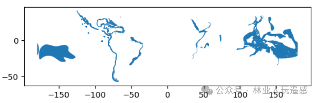
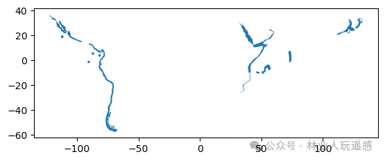
Shapefile data can be saved using gpd.to_file(). We first select a portion of the data using index slicing, and then use this function to write the selected data to a new Shapefile.
# Adjust the path according to actual conditions
out_file_path = r"...\DAMSELFISH_distributions_SELECTION.shp"
selection = data[0:50]
selection.to_file(out_file_path)
The selected data is shown in the figure below.
02
—
Geometric Objects in Geopandas
Geopandas utilizes geometric objects from Shapely. Geometric information is typically stored in a column named “geometry”. This is the default column name used in geopandas for storing geometric information.
Let’s check the first 5 rows of the “geometry” column.
In [7]: data['geometry'].head()Out[7]: 0 POLYGON ((-115.64375 29.71392, -115.61585 29.6...1 POLYGON ((-105.58995 21.89340, -105.56483 21.8...2 POLYGON ((-111.15962 19.01536, -111.15948 18.9...3 POLYGON ((-80.86500 -0.77894, -80.75930 -0.833...4 POLYGON ((-67.33922 -55.67610, -67.33755 -55.6...Name: geometry, dtype: geometrySince the data is stored as Shapely objects, we can use all the functionalities of the Shapely module.
We can check the area of the first 5 polygons.
In [8]: selection = data[0:5]We can iterate through the selected rows using the specific .iterrows() function in geopandas and print the area of each polygon.
In [9]: for index, row in selection.iterrows(): ...: poly_area = row['geometry'].area ...: print("Polygon area at index {0} is: {1:.3f}".format(index, poly_area)) ...: Polygon area at index 0 is: 19.396Polygon area at index 1 is: 6.146Polygon area at index 2 is: 2.697Polygon area at index 3 is: 87.461Polygon area at index 4 is: 0.001All functionalities of pandas can be directly used in geopandas without separately calling pandas, as geopandas is an extension of pandas.
Next, we will create a new column in geopandas to calculate and store the area of each polygon. In geopandas, the area of polygons can be calculated using the GeoDataFrame.area property.
In [10]: data['area'] = data.areaLet’s check the first two rows of the area column.
In [11]: data['area'].head(2)Out[11]: 0 19.3962541 6.145902Name: area, dtype: float64These values are consistent with the results we saw earlier when iterating through the rows. We can use common pandas functions to check the minimum and maximum values of these areas.
In [12]: max_area = data['area'].max()
In [13]: mean_area = data['area'].mean()
In [14]: print("Max area: {:.2f}\nMean area: {:.2f}".format(round(max_area, 2), round(mean_area, 2)))Max area: 1493.20Mean area: 19.96
03
—
Creating Geometric Objects in Geopandas
Since geopandas utilizes Shapely geometric objects, we can create a Shapefile from scratch by passing Shapely geometric objects into a GeoDataFrame, which allows for easy conversion of text files containing coordinates into Shapefiles.
First, we create an empty GeoDataFrame.
import geopandas as gpdfrom shapely.geometry import Polygon
newdata = gpd.GeoDataFrame()
Next, we create a new column named “geometry” to store our Shapely objects.
In [16]: newdata['geometry'] = NoneWe then create a Shapely polygon and insert it into our geopandas.
In [18]: coordinates = [(26.722117, 58.380184), (26.724853, 58.380676), (26.724961, 58.380518), (26.722372, 58.379933)]
In [19]: poly = Polygon(coordinates)
We insert this polygon into the “geometry” column of newdata.
In [21]: newdata.loc[0, 'geometry'] = polyNext, we add a column named “Location” and fill it with the text “Square”.
In [23]: newdata.loc[0, 'Location'] = 'Square'Before exporting the data, we need to determine the coordinate reference system (projection) for the GeoDataFrame.
The GeoDataFrame has a property called .crs that shows the coordinate system of the data. Since we are creating the data from scratch, the value of this property is currently empty (None).
In [25]: print(newdata.crs)NoneThe from_epsg() function from the fiona package can be used to set the coordinate system (crs) for the GeoDataFrame.
In [26]: from fiona.crs import from_epsg
In [27]: newdata.crs = from_epsg(4326)
Let’s check the data.
# If using IDE, explicitly call plt.show()
# If using a notebook and have run %matplotlib inline, the image will display correctly
In [29]: newdata.plot()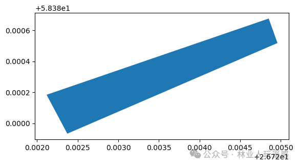 Finally, we can use the .to_file() function to export the data. The usage of this function is similar to that in numpy or pandas, but here we only need to provide the output path for the Shapefile.
# Fill in the path according to local conditions
out_file = ".../Example.shp"
newdata.to_file(out_file)
We have just created a Shapefile from scratch. Similar methods can be used for other cases, such as reading coordinates from text files (like point coordinates) and creating Shapefiles based on those coordinates.
04
—
Saving Multiple Shapefiles
A very useful function in Geopandas is groupby(). With the groupby() function, we can group data based on values in selected columns.
We will group different fish species in DAMSELFISH_distribution.shp and export them as separate Shapefiles.
In [30]: grouped = data.groupby('BINOMIAL')The groupby() function returns an object called DataFrameGroupBy, which is similar to a list of keys and values (like a dictionary structure), and we can iterate over it.
In [32]: for key, values in grouped: ....: individual_fish = values ....: print(key)Let’s check the data type of this grouped object and what the key variable contains.
In [33]: individual_fishOut[33]:        ID_NO                BINOMIAL  ORIGIN COMPILER  YEAR
27  154915.0  Teixeirichthys jordani       1     None  2012
28  154915.0  Teixeirichthys jordani       1     None  2012
29  154915.0  Teixeirichthys jordani       1     None  2012
30  154915.0  Teixeirichthys jordani       1     None  2012
31  154915.0  Teixeirichthys jordani       1     None  2012
32  154915.0  Teixeirichthys jordani       1     None  2012
33  154915.0  Teixeirichthys jordani       1     None  2012                                                CITATION SOURCE DIST_COMM ISLAND
27  Red List Index (Sampled Approach), Zoological ...   None      None   None
28  Red List Index (Sampled Approach), Zoological ...   None      None   None
29  Red List Index (Sampled Approach), Zoological ...   None      None   None
30  Red List Index (Sampled Approach), Zoological ...   None      None   None
31  Red List Index (Sampled Approach), Zoological ...   None      None   None
32  Red List Index (Sampled Approach), Zoological ...   None      None   None
33  Red List Index (Sampled Approach), Zoological ...   None      None   None      SUBSPECIES  ... KINGDOM_NA PHYLUM_NAM      CLASS_NAME   ORDER_NAME
27       None  ...   ANIMALIA   CHORDATA  ACTINOPTERYGII  PERCIFORMES
28       None  ...   ANIMALIA   CHORDATA  ACTINOPTERYGII  PERCIFORMES
29       None  ...   ANIMALIA   CHORDATA  ACTINOPTERYGII  PERCIFORMES
30       None  ...   ANIMALIA   CHORDATA  ACTINOPTERYGII  PERCIFORMES
31       None  ...   ANIMALIA   CHORDATA  ACTINOPTERYGII  PERCIFORMES
32       None  ...   ANIMALIA   CHORDATA  ACTINOPTERYGII  PERCIFORMES
33       None  ...   ANIMALIA   CHORDATA  ACTINOPTERYGII  PERCIFORMES          FAMILY_NAM      GENUS_NAME SPECIES_NA CATEGORY
27  POMACENTRIDAE  Teixeirichthys    jordani       LC
28  POMACENTRIDAE  Teixeirichthys    jordani       LC
29  POMACENTRIDAE  Teixeirichthys    jordani       LC
30  POMACENTRIDAE  Teixeirichthys    jordani       LC
31  POMACENTRIDAE  Teixeirichthys    jordani       LC
32  POMACENTRIDAE  Teixeirichthys    jordani       LC
33  POMACENTRIDAE  Teixeirichthys    jordani       LC                                                geometry       area  27  POLYGON ((121.63003 33.04249, 121.63219 33.042...  38.671198
28  POLYGON ((32.56219 29.97489, 32.56497 29.96967...  37.445735
29  POLYGON ((130.90521 34.02498, 130.90710 34.022...  16.939460
30  POLYGON ((56.32233 -3.70727, 56.32294 -3.70872...  10.126967
31  POLYGON ((40.64476 -10.85502, 40.64600 -10.855...   7.760303
32  POLYGON ((48.11258 -9.33510, 48.11406 -9.33614...   3.434236
33  POLYGON ((51.75404 -9.21679, 51.75532 -9.21879...   2.408620
[7 rows x 25 columns]
In [34]: type(individual_fish)Out[34]: geopandas.geodataframe.GeoDataFrame
In [35]: print(key)Teixeirichthys jordani
From here we can see that the individual_fish variable now contains all rows for the fish named Teixeirichthys jordani. The index numbers correspond to the row numbers in the data variable.
From the above example, we can see that each group of data is now separated into individual GeoDataFrames, and we can use the key variable to create output file paths to export these data as Shapefiles.
We will export these fish species as separate Shapefiles.
import os# Adjust the file path according to local conditions
result_folder = ".../results"
for key, values in grouped:    # Format the file name (replace spaces with underscores)    updated_key = key.replace(" ", "_")    out_name = updated_key + ".shp"    # Print process information    print( "Processing: {}".format(out_name) )    # Create an output path by joining the two folder names without using slashes or backslashes    outpath = os.path.join(result_folder, out_name)    # Export data    values.to_file(outpath)
Now we have saved these individual fish species into their respective Shapefiles, and the file names are based on the species names. This type of grouping operation is very convenient when working with Shapefiles, as performing similar operations manually can be very tedious and error-prone.