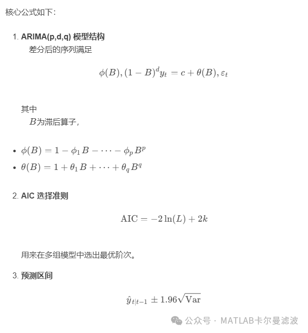
Using the ARIMA model to model and predict GNSS positioning errors in urban canyon environments. GNSS errors often exhibit time-related trends, seasonal components, and random disturbances. This code constructs a simulated error sequence that includes trends, seasonality, and noise, and divides it into training and testing sets. It then iterates through multiple sets of ARIMA(p,d,q) parameter combinations, automatically selecting the optimal model based on the AIC criterion. After establishing the optimal model, it predicts the errors for the testing period and provides a 95% confidence interval. The results include: original data, predicted results, and prediction error curves.<span>The code is original and not AI-generated, with comments in Chinese.</span>

To evaluate prediction performance, the code calculates the Mean Absolute Error (MAE), Root Mean Square Error (RMSE), and Mean Absolute Percentage Error (MAPE), and outputs key parameters such as the AR and MA coefficients and variance of the model. The script finally presents a point-by-point comparison of some predictions and actual errors in tabular form, facilitating a quick assessment of the model’s applicability in positioning error prediction scenarios.

Results

Original actual data: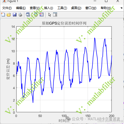

Comparison of predicted results with actual curves: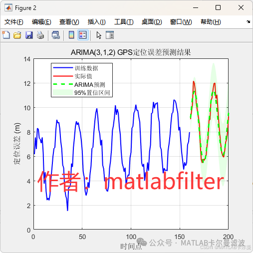Difference between predictions and actual values: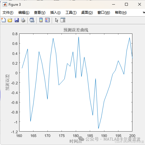

Command line output results: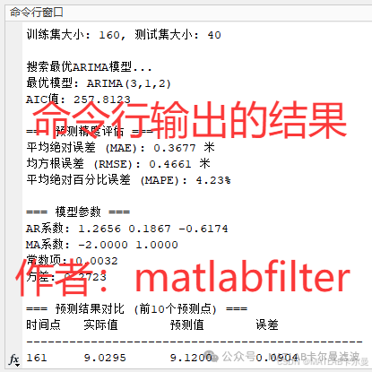

MATLAB Source Code

Part of the code is as follows:

%% ARIMA model for GNSS positioning error prediction
% Background: GNSS receiver positioning error prediction in urban canyon environments
% Author: matlabfilter, for MATLAB code customization and explanation
% 2025-11-23/Ver1: Added comparison

clear; clc; close all;
rng(0);% Set random seed for reproducibility

%% Simulate GNSS positioning error data
% Length of time series
n =200;
t =1:n;

% Simulate GNSS positioning error (meters)
% Includes trend, seasonal, and random noise
trend =0.02* t;% Slowly increasing trend (e.g., satellite geometry changes)
seasonal =3*sin(2*pi*t/20);% Periodic fluctuations (e.g., multipath effects)
noise =randn(n,1)'*0.4;% Random noise
gps_error = trend + seasonal + noise +5;% Baseline error of 5 meters

% Convert to column vector
gps_error = gps_error';

%% Data visualization
figure;
plot(t, gps_error,'b-','LineWidth',1.5);
xlabel('Time Point');
ylabel('Positioning Error (m)');
title('Original GNSS Positioning Error Time Series');
grid on;


%% Split into training and testing sets
train_ratio =0.8;
train_size =floor(length(gps_error)* train_ratio);
train_data =gps_error(1:train_size);
test_data =gps_error(train_size+1:end);

fprintf('Training set size: %d, Testing set size: %d\n', train_size,length(test_data));

%% Model identification and order determination
% Try different ARIMA model parameters
p_values =0:3;% AR order
d_values =0:1;% Differencing order
q_values =0:3;% MA order

best_aic =inf;
best_model =[];
best_params =[0,0,0];

Complete code download link:

Or click on the “Read Original” link at the end to navigate.

<span>If you need assistance or have customization requirements for navigation and positioning filtering related code, please click the card below to contact the author.</span>

Please open in the WeChat client