1. Overview

1.1 Creating a Grid of Axes

1.1.1 subplots

This function has been previously learned, and it is the main function used to create a grid of Figures and Axes. It creates and places all Axes in the Figure at once and returns an array of objects containing Axes handles.

1.1.2 subplot_mosaic

A simple method to create a grid of Figures and Axes, which adds flexibility for Axes to span rows or columns. The returned Axes will be in the form of a labeled dictionary instead of an array.

1.1.3 SubFigure

Used to create subfigures within a Figure.

1.2 Underlying Tools

The underlying tools here mainly refer to the concepts of GridSpec and SubplotSpec.

1.2.1 GridSpec

Specifies the grid geometry for placing subplots. It requires setting the number of rows and columns in the grid, and layout parameters for the subplots (e.g., left, right, etc.) can be adjusted (optional).

1.2.2 SubplotSpec

Specifies the position of the subplot within GridSpec.

1.3 Adding a Single Axes at a Time

The above functions create all Axes in a single function call, while adding one Axes at a time, although not very elegant or flexible, can be useful for interactive plotting or placing Axes in custom locations. The following methods implement adding a single Axes at a time:

1.3.1 add_axes

Adds a single Axes at a specified position in the Figure, scaled according to [left, bottom, width, height].

1.3.2 subplot or Figure.add_subplot

Adds a single subplot to the figure, indexing starts from 1 (inherited from Matlab). It can span columns and rows by specifying the range of grid cells.

1.3.3 subplot2grid

Similar to pyplot.subplot, but uses zero-based indexing and two-dimensional Python slicing to select cells.

1.3.4 Example

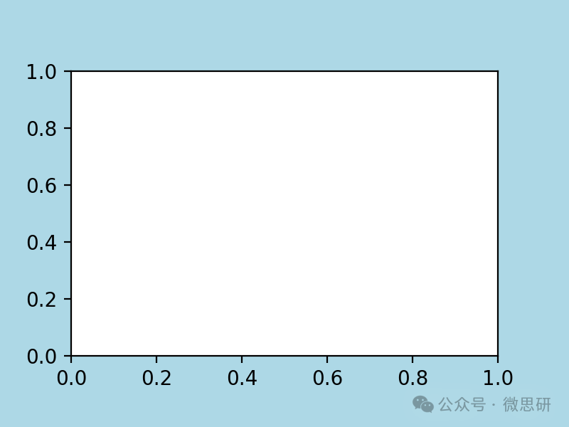
Here is a simple example of manually adding an Axes ax, where we add a 3-inch x 2-inch Axes to a 4-inch x 3-inch figure. Note that the position of the subplot is defined based on [left, bottom, width, height], and is expressed in normalized units of the figure:

import matplotlib.pyplot as plt
import numpy as np

w, h = 4, 3
margin = 0.5
fig = plt.figure(figsize=(w, h), facecolor='lightblue')
ax = fig.add_axes([margin / w, margin / h, (w - 2 * margin) / w,
                      (h - 2 * margin) / h])

Basic Python Plotting: How to Arrange Multiple Axes in a Single Figure?

2. Advanced Methods for Creating Axes Grids

2.1 Basic 2×2 Grid

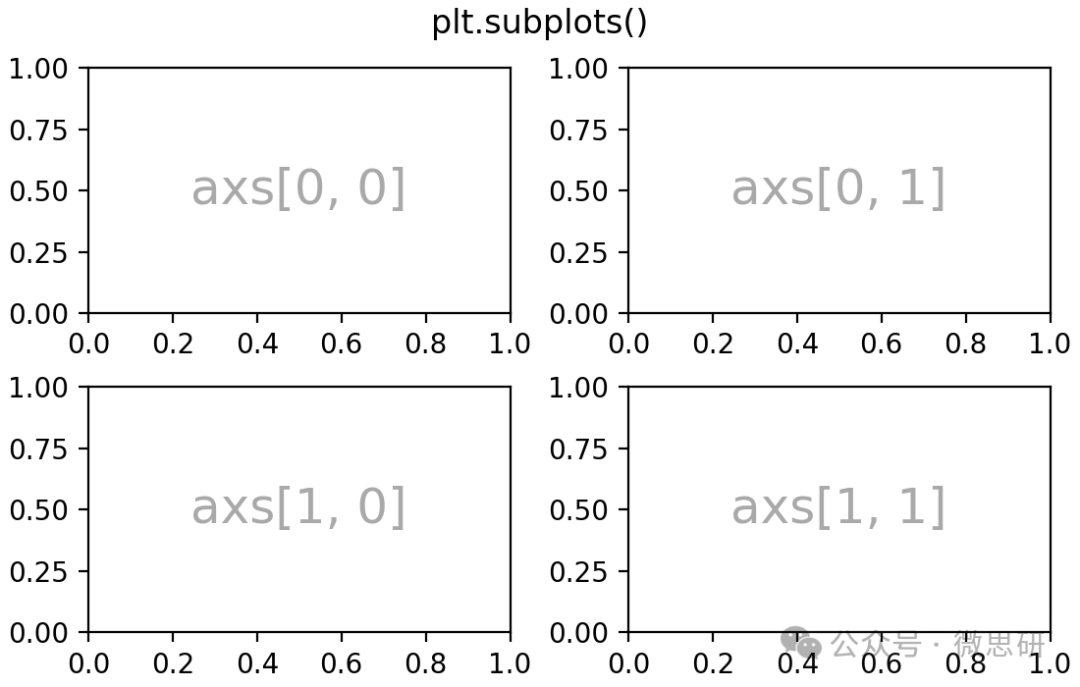
A basic 2×2 Axes grid can be created using subplots, which returns a Figure instance and an array of Axes objects. The Axes objects can be used to access methods for adding Artists to the axes. Here we use annotate, but it could be plot, pcolormesh, etc.

fig, axs = plt.subplots(ncols=2, nrows=2, figsize=(5.5, 3.5),
                        layout="constrained")
# add an artist, in this case a nice label in the middle...
for row in range(2):
    for col in range(2):
        axs[row, col].annotate(f'axs[{row}, {col}]', (0.5, 0.5),
                               transform=axs[row, col].transAxes,
                               ha='center', va='center', fontsize=18,
                               color='darkgrey')
fig.suptitle('plt.subplots()')

Next, we will annotate many Axes, for which we will encapsulate the annotation method instead of writing a long annotation code each time it is needed:

def annotate_axes(ax, text, fontsize=18):
    ax.text(0.5, 0.5, text, transform=ax.transAxes,
            ha="center", va="center", fontsize=fontsize, color="darkgrey")

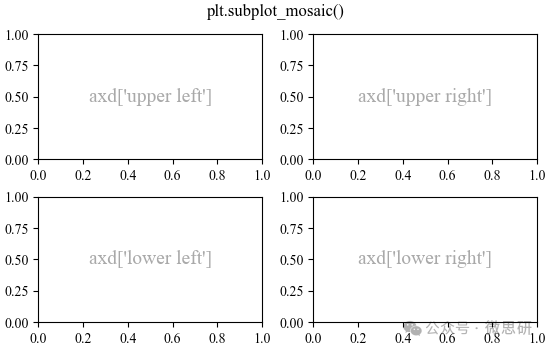
Using subplot_mosaic can achieve the same effect, but the return type is a dictionary instead of an array, allowing users to assign useful meanings to the dictionary’s keys. Here we provide two lists, each representing a row, with each element in the list representing a column key. (Note the use of “!r” in the code below, which is mainly used to output the quotes of the string, equivalent to the repr() method)

fig, axd = plt.subplot_mosaic([['upper left', 'upper right'],
                               ['lower left', 'lower right']],
                              figsize=(5.5, 3.5), layout="constrained")
for k, ax in axd.items():
    annotate_axes(ax, f'axd[{k!r}]', fontsize=14)
fig.suptitle('plt.subplot_mosaic()')

2.2 Axes Grid with Fixed Aspect Ratio

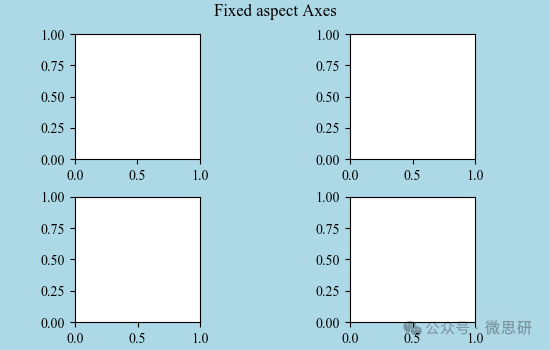
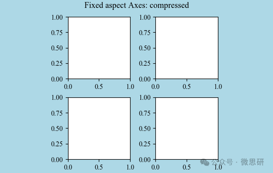
Axes with a fixed aspect ratio are common in images or maps. However, they pose challenges for layout since the size of the axes is constrained in two ways—they must fit the figure size and maintain a fixed aspect ratio.This can lead to large gaps between Axes by default, as shown:

fig, axs = plt.subplots(2, 2, layout="constrained",
                        figsize=(5.5, 3.5), facecolor='lightblue')
for ax in axs.flat:
    ax.set_aspect(1)
fig.suptitle('Fixed aspect Axes')

There are large gaps between the subplots:

One way to solve this problem is to use layout="compressed":

fig, axs = plt.subplots(2, 2, layout="compressed", figsize=(5.5, 3.5),
                        facecolor='lightblue')
for ax in axs.flat:
    ax.set_aspect(1)
fig.suptitle('Fixed aspect Axes: compressed')

2.3 Axes Spanning Rows or Columns in a Grid

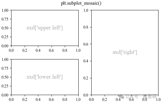
This means that the subplots are no longer evenly distributed in rows and columns, but rather resemble the difference between SQL and NoSQL storage methods, for example, the entire Figure is divided into three parts: upper left, lower left, and right. The most common implementation method is subplot_mosaic:

fig, axd = plt.subplot_mosaic([['upper left', 'right'],
                               ['lower left', 'right']],
                              figsize=(5.5, 3.5), layout="constrained")
for k, ax in axd.items():
    annotate_axes(ax, f'axd[{k!r}]', fontsize=14)
fig.suptitle('plt.subplot_mosaic()')

2.4 Variable Width and Height in a Grid

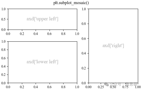
subplots and subplot_mosaic both allow the use of the gridspec_kw keyword argument to set different heights for rows and widths for columns in the grid. The spacing parameters accepted by GridSpec can be passed to subplots and subplot_mosaic:

gs_kw = dict(width_ratios=[1.4, 1], height_ratios=[1, 2])
fig, axd = plt.subplot_mosaic([['upper left', 'right'],
                               ['lower left', 'right']],
                              gridspec_kw=gs_kw, figsize=(5.5, 3.5),
                              layout="constrained")
for k, ax in axd.items():
    annotate_axes(ax, f'axd[{k!r}]', fontsize=14)
fig.suptitle('plt.subplot_mosaic()')

2.5 Nested Axes Layout

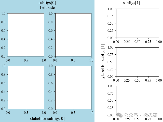
Implemented using Figure.subfigures:

fig = plt.figure(layout="constrained")
subfigs = fig.subfigures(1, 2, wspace=0.07, width_ratios=[1.5, 1.])
axs0 = subfigs[0].subplots(2, 2)
subfigs[0].set_facecolor('lightblue')
subfigs[0].suptitle('subfigs[0]\nLeft side')
subfigs[0].supxlabel('xlabel for subfigs[0]')

axs1 = subfigs[1].subplots(3, 1)
subfigs[1].suptitle('subfigs[1]')
subfigs[1].supylabel('ylabel for subfigs[1]')

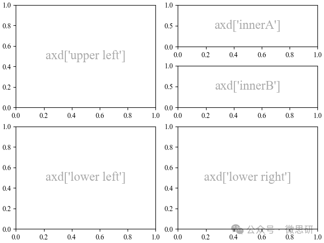
It is also possible to use subplot_mosaic with nested lists to nest Axes. This method does not use subfigures like the above, thus lacking the ability to add suptitle, supxlabel, etc. for each subplot. Instead, it is a convenient encapsulation of the subgridspec method described below:

inner = [['innerA'],
         ['innerB']]
outer = [['upper left',  inner],
          ['lower left', 'lower right']]

fig, axd = plt.subplot_mosaic(outer, layout="constrained")
for k, ax in axd.items():
    annotate_axes(ax, f'axd[{k!r}]')

3. Other Methods

Internally, the arrangement of the Axes grid is controlled by creating instances of GridSpec and SubplotSpec. GridSpec defines a (possibly uneven) grid of cells. Indexing into GridSpec will return a SubplotSpec that spans one or more grid cells, which can be used to specify the position of the Axes.

The following example shows how to arrange Axes using the low-level method through the GridSpec object.

3.1 Basic 2×2 Grid

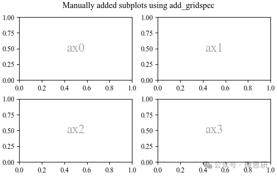
We can create a 2×2 grid in the same way:plt.subplots(2, 2):

fig = plt.figure(figsize=(5.5, 3.5), layout="constrained")
spec = fig.add_gridspec(ncols=2, nrows=2)

ax0 = fig.add_subplot(spec[0, 0])
annotate_axes(ax0, 'ax0')

ax1 = fig.add_subplot(spec[0, 1])
annotate_axes(ax1, 'ax1')

ax2 = fig.add_subplot(spec[1, 0])
annotate_axes(ax2, 'ax2')

ax3 = fig.add_subplot(spec[1, 1])
annotate_axes(ax3, 'ax3')

fig.suptitle('Manually added subplots using add_gridspec')

3.2 Axes Spanning Rows or Columns in a Grid

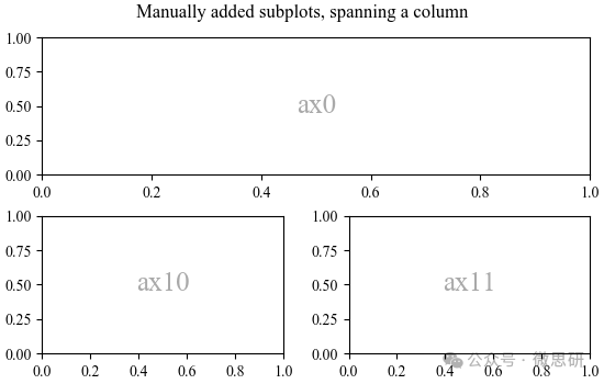
We can index the spec array using NumPy slicing, and the new Axes will span the slice. This is equivalent to:fig, axd = plt.subplot_mosaic([['ax0', 'ax0'], ['ax1', 'ax2']], ...):

fig = plt.figure(figsize=(5.5, 3.5), layout="constrained")
spec = fig.add_gridspec(2, 2)

ax0 = fig.add_subplot(spec[0, :])
annotate_axes(ax0, 'ax0')

ax10 = fig.add_subplot(spec[1, 0])
annotate_axes(ax10, 'ax10')

ax11 = fig.add_subplot(spec[1, 1])
annotate_axes(ax11, 'ax11')

fig.suptitle('Manually added subplots, spanning a column')

3.3 Manually Adjusting GridSpec Layout

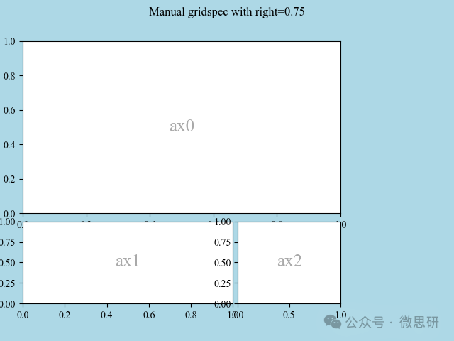
When explicitly using GridSpec, the layout parameters of the subplots created from GridSpec can be adjusted. It is important to note that this option is incompatible with constrained layout or ignoring left and adjusting subplot sizes to fill the figure using Figure.tight_layout. Typically, this manual placement requires iteration to ensure that the Axes scale labels do not overlap with the Axes.

These spacing parameters can also be passed as gridspec_kw parameters to subplots and subplot_mosaic.

fig = plt.figure(layout=None, facecolor='lightblue')
gs = fig.add_gridspec(nrows=3, ncols=3, left=0.05, right=0.75,
                      hspace=0.1, wspace=0.05)
ax0 = fig.add_subplot(gs[:-1, :])
annotate_axes(ax0, 'ax0')
ax1 = fig.add_subplot(gs[-1, :-1])
annotate_axes(ax1, 'ax1')
ax2 = fig.add_subplot(gs[-1, -1])
annotate_axes(ax2, 'ax2')
fig.suptitle('Manual gridspec with right=0.75')

3.4 Using SubplotSpec for Nested Layouts

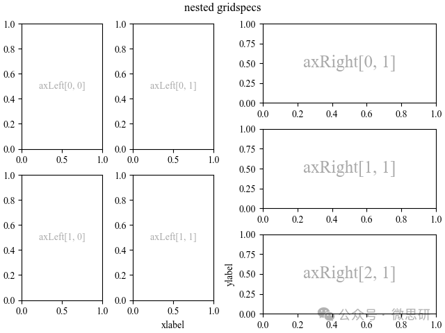
You can create nested layouts similar to subfigures using subgridspec:

fig = plt.figure(layout="constrained")
gs0 = fig.add_gridspec(1, 2)

gs00 = gs0[0].subgridspec(2, 2)
gs01 = gs0[1].subgridspec(3, 1)

for a in range(2):
    for b in range(2):
        ax = fig.add_subplot(gs00[a, b])
        annotate_axes(ax, f'axLeft[{a}, {b}]', fontsize=10)
        if a == 1 and b == 1:
            ax.set_xlabel('xlabel')
for a in range(3):
    ax = fig.add_subplot(gs01[a])
    annotate_axes(ax, f'axRight[{a}, {b}]')
    if a == 2:
        ax.set_ylabel('ylabel')

fig.suptitle('nested gridspecs')

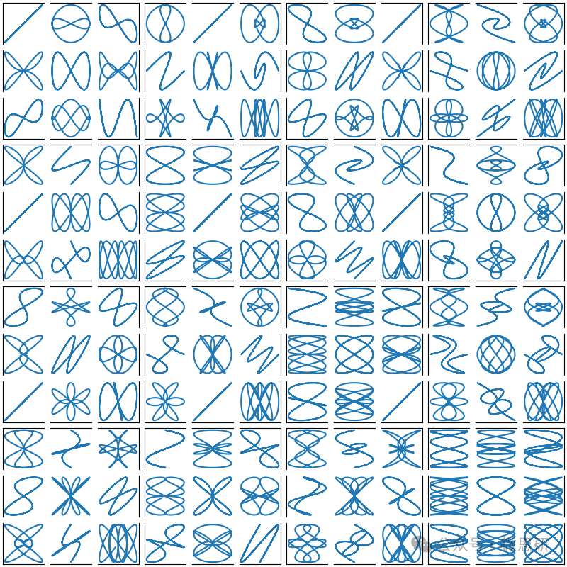
Below is a more complex nested GridSpec example: we create an outer grid of 4×4, with each cell containing an inner grid of 3×3 Axes. We outline the outer 4×4 grid by hiding the corresponding Axes spines in each inner 3×3 grid:

def squiggle_xy(a, b, c, d, i=np.arange(0.0, 2*np.pi, 0.05)):
    return np.sin(i*a)*np.cos(i*b), np.sin(i*c)*np.cos(i*d)

fig = plt.figure(figsize=(8, 8), layout='constrained')
outer_grid = fig.add_gridspec(4, 4, wspace=0, hspace=0)

for a in range(4):
    for b in range(4):
        # gridspec inside gridspec
        inner_grid = outer_grid[a, b].subgridspec(3, 3, wspace=0, hspace=0)
        axs = inner_grid.subplots()  # Create all subplots for the inner grid.
        for (c, d), ax in np.ndenumerate(axs):
            ax.plot(*squiggle_xy(a + 1, b + 1, c + 1, d + 1))
            ax.set(xticks=[], yticks=[])

# show only the outside spines
for ax in fig.get_axes():
    ss = ax.get_subplotspec()
    ax.spines.top.set_visible(ss.is_first_row())
    ax.spines.bottom.set_visible(ss.is_last_row())
    ax.spines.left.set_visible(ss.is_first_col())
    ax.spines.right.set_visible(ss.is_last_col())

plt.show()

4. References

https://matplotlib.org/stable/api/_as_gen/matplotlib.pyplot.subplots.html#matplotlib.pyplot.subplots
https://matplotlib.org/stable/api/_as_gen/matplotlib.pyplot.subplot_mosaic.html#matplotlib.pyplot.subplot_mosaic
https://matplotlib.org/stable/api/_as_gen/matplotlib.gridspec.GridSpecFromSubplotSpec.html#matplotlib.gridspec.GridSpecFromSubplotSpec