💥💥💞💞Welcome to this blog❤️❤️💥💥
🏆Advantages of the Blogger:🌞🌞🌞The blog content aims to be logically coherent and clear for the convenience of readers.
⛳️Motto:Those who travel a hundred miles are halfway at ninety.
⛳️Gift to Readers
👨💻Conducting research involves a profound system of thought, requiring researchers to be logical and diligent, but effort alone is not enough; often leveraging resources is more important. Additionally, one must have innovative and inspiring points of view. When a philosophy teacher asks you what science is or what electricity is, do not find these questions amusing. Philosophy is the mother of science; it seeks ultimate questions and looks for those self-evident questions that only children would ask but you cannot answer. Readers are advised to browse in order to avoid suddenly falling into a dark maze without finding their way back. It may not reveal all the answers to your questions, but if it can evoke clouds of doubt in your mind, it may create a beautiful sunset. If it brings you a spiritual downpour, take the opportunity to brush off the dust that has settled on your ‘lying flat’ state.
Perhaps, after the rain, the sky will be clearer…….🔎🔎🔎
💥1 Overview
The SSTL (Signalized Intersection Traffic Light) standard is a specification used to control signalized intersections, aimed at improving traffic efficiency, reducing congestion, and lowering accident rates. Studying the application of the SSTL standard at signalized intersections can help traffic management departments optimize traffic signal control schemes and enhance the operational efficiency of traffic flow.
Research on Controlling Signalized Intersections Using SSTL Standards
1. Introduction
With the acceleration of urbanization, traffic congestion in cities has become increasingly severe. As key nodes in urban traffic, the management efficiency of signalized intersections directly affects the operation of the entire traffic system. The SSTL (Signalized Intersection Traffic Light) standard, as an advanced signal control technology, aims to optimize signal light control schemes to improve traffic efficiency, reduce congestion, and lower accident rates. This article aims to explore the application of the SSTL standard at signalized intersections, providing references for traffic management departments to optimize traffic signal control schemes.
2. Overview of SSTL Standards
The SSTL standard is a specification for controlling signalized intersections that employs advanced signal control technology. It dynamically adjusts the timing intervals and green light durations of traffic signals to achieve more efficient and safer traffic flow. The core features of the SSTL standard include:
- Dynamic Adjustment: Real-time adjustment of signal timing intervals and green light durations based on changes in traffic flow and vehicle counts, minimizing vehicle queue and wait times.
- Split Cycle: Dividing the cycle into two phases, each assigned different green light durations to ensure sufficient green time for each direction.
- Offset Optimization: Coordinating the timing intervals between different traffic signals to reduce vehicle queue and wait times.
- Signal Logic: Intelligently allocating green light durations to each direction based on changes in traffic flow.
3. Research on the Application of SSTL Standards at Signalized Intersections
1. Traffic Flow Survey and Analysis
By surveying and analyzing the traffic flow around signalized intersections, we can understand the traffic flow conditions during different time periods, including vehicle types, travel directions, and flow volumes. This data provides foundational support for developing reasonable signal control schemes.
2. Signal Control Scheme Design
Based on the results of the traffic flow survey and the characteristics of the intersection, design a signal control scheme suitable for that intersection. The design content includes, but is not limited to:
- Signal Timing: Determining the duration of green, yellow, and red lights for each direction.
- Phase Settings: Reasonably setting phases based on traffic flow and road conditions to ensure smooth traffic flow.
- Split Cycle and Offset Optimization: Applying split cycle and offset optimization techniques to dynamically adjust signal timing intervals, reducing vehicle queue and wait times.
3. Simulation Analysis
Using traffic simulation software (such as VISSIM, SUMO, etc.) to simulate and analyze the designed signal control scheme. Through simulation, evaluate the effectiveness of the scheme under different traffic flow conditions, including vehicle queue lengths, delay times, and throughput capacity. Based on the simulation results, optimize and adjust the signal control scheme.
4. Field Verification and Adjustment
Verify the designed signal control scheme in actual traffic environments. By installing traffic detectors, cameras, and other equipment, collect actual traffic data to assess the effectiveness and reliability of the signal control scheme. Adjust and optimize based on actual results to ensure the signal control scheme can adapt to real traffic demands.
4. Case Study
Taking a typical signalized intersection in a certain city as an example, apply the SSTL standard for signal control optimization.
1. Traffic Flow Survey
Collect traffic flow data at the intersection during different time periods through manual observation and video capture technology. Analysis shows that the intersection experiences high traffic flow during morning and evening peak hours, with significant directional imbalance.
2. Signal Control Scheme Design
Based on the traffic flow survey results, design the following signal control scheme:
- Signal Timing: Appropriately extend green light durations during peak hours to reduce red light wait times.
- Phase Settings: Set four phases to control straight and left-turning vehicles in both east-west and north-south directions based on traffic flow and road conditions.
- Split Cycle and Offset Optimization: Apply split cycle technology to divide the cycle into two phases, each assigned different green light durations. Simultaneously, apply offset optimization technology to coordinate the timing intervals between different signals, reducing vehicle queue and wait times.
3. Simulation Analysis
Utilize VISSIM software to simulate the designed signal control scheme. Simulation results indicate that the optimized signal control scheme significantly reduces vehicle queue lengths and delay times, improving the intersection’s throughput capacity.
4. Field Verification and Adjustment
Verify the designed signal control scheme in actual traffic environments. By installing traffic detectors, cameras, and other equipment, collect actual traffic data. Evaluation results show that the optimized signal control scheme achieved good results in practice, with reductions in both vehicle queue lengths and delay times. Additionally, minor adjustments were made to the signal control scheme based on actual performance to further enhance its adaptability and effectiveness.
5. Conclusion and Outlook
1. Research Conclusions
By applying the SSTL standard for signal control optimization at signalized intersections, traffic efficiency can be significantly improved, congestion reduced, and accident rates lowered. The dynamic adjustment, split cycle, offset optimization, and signal logic features of the SSTL standard enable it to meet the demands of varying traffic flow conditions, achieving more efficient and safer traffic flow.
2. Research Outlook
Future research can further explore the application effects of the SSTL standard at other types of intersections (such as roundabouts, grade-separated intersections, etc.). Additionally, it can investigate how to integrate the SSTL standard with intelligent transportation systems, vehicle-road collaboration, and autonomous driving technologies to achieve higher-level traffic signal control optimization. Furthermore, cross-regional and cross-city signal control coordination optimization research can be conducted to further enhance the operational efficiency of the entire traffic system.
📚2 Operational Results
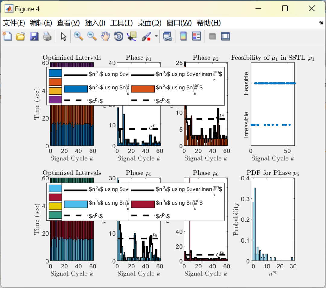
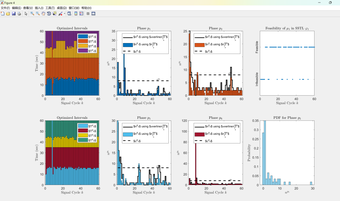
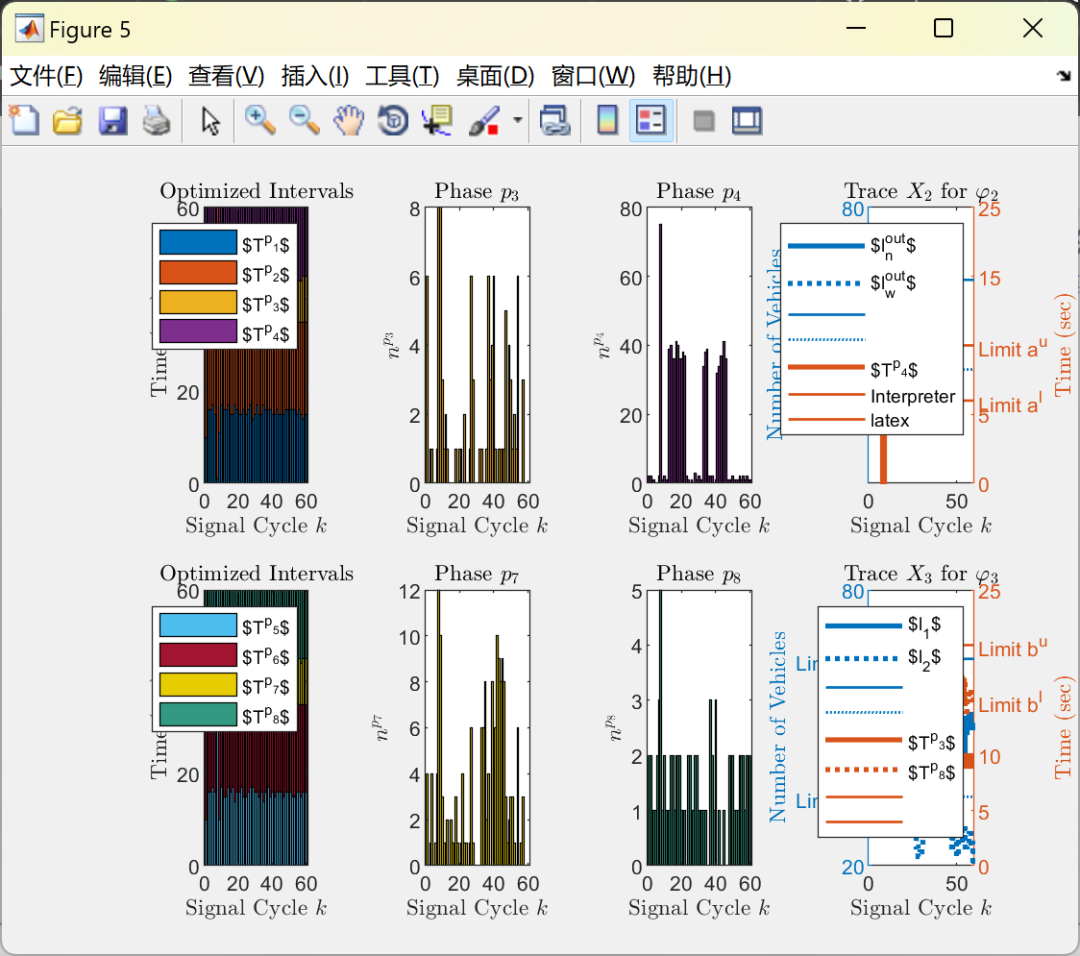
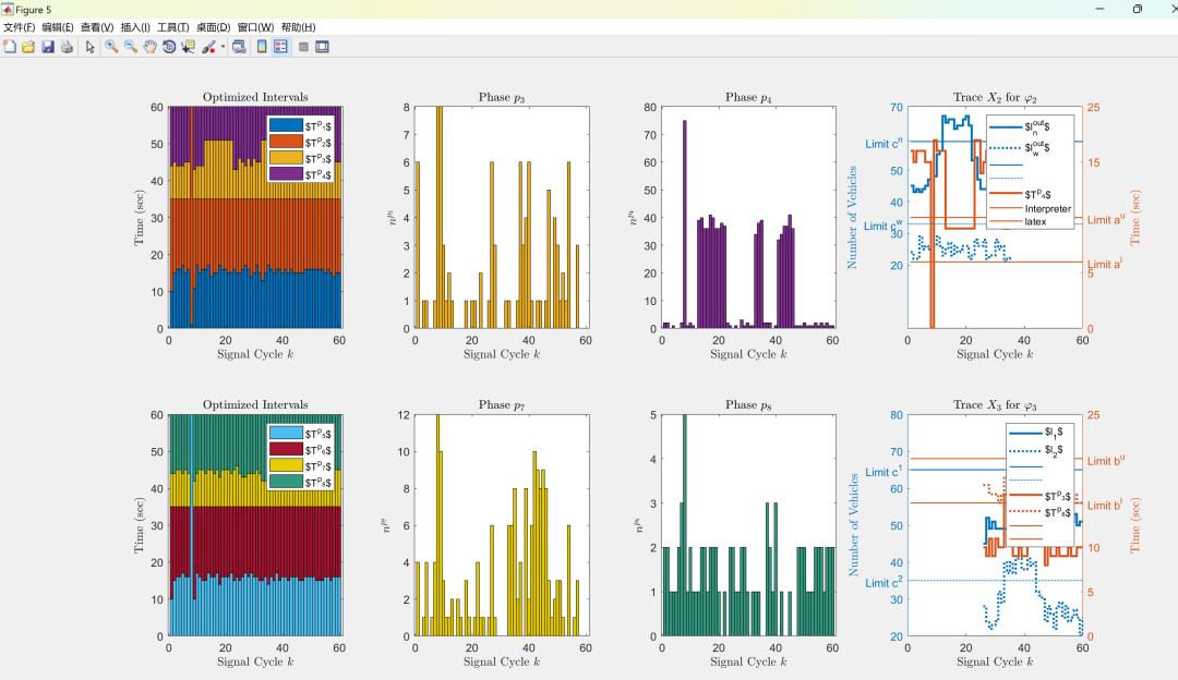
Partial Code:
subplot(2,4,4); plot(SSTLPhi1FeasibilityUB,'.','MarkerSize',10);
title({'Feasibility of $\mu_{1}$ in SSTL $\varphi_{1}$'},'Interpreter','latex');
xlabel('Signal Cycle $k$','Interpreter','latex');
ylim([-0.5,1.5]);
yticks([0 1]);
yticklabels({'Infeasible','Feasible'});
ytickangle(90);
subplot(2,4,5); BarGraphp5p6p7p8 = bar(BarGraphMatrixp5p6p7p8, 'stacked','BarWidth',1);
BarGraphp5p6p7p8(1).FaceColor = [0.3010 0.7450 0.9330]; BarGraphp5p6p7p8(2).FaceColor = [0.6350 0.0780 0.1840];
BarGraphp5p6p7p8(3).FaceColor = [0.9 0.8 0]; BarGraphp5p6p7p8(4).FaceColor = [.2 .6 .5];
legend('$T^{p_{5}}$','$T^{p_{6}}$','$T^{p_{7}}$','$T^{p_{8}}$','Interpreter','latex');
title('Optimized Intervals','Interpreter','latex');
xlabel('Signal Cycle $k$','Interpreter','latex');
ylabel('Time (sec)','Interpreter','latex');
subplot(2,4,6); stairs(0.5:1:59.5,OptimalNNp5Green,'k','LineWidth',2);
hold on;
bar(ObservedNNp5Green,'FaceColor',[0.3010 0.7450 0.9330],'BarWidth',1);
title('Phase $p_{5}$','Interpreter','latex');
xlabel('Signal Cycle $k$','Interpreter','latex');
ylabel('$n^{p_{5}}$','Interpreter','latex');
ylim([0,30]);
hold on;
plot(NNp5GreenLimit*ones(1,NoSignalCycles),'--','Color','k','LineWidth',2);
legend('$n^{p_{5}}$ using $\overline{n}_{l_{n}^{in}}^{ran}$','$n^{p_{5}}$ using $n_{l_{n}^{in}}^{ran}$','$c^{p_{5}}$','Interpreter','latex');
text(45,NNp5GreenLimit+0.7,{'$c^{p_{5}}$'},'Interpreter','latex');
subplot(2,4,7); stairs(0.5:1:59.5,OptimalNSp6Green,'k','LineWidth',2);
hold on;
bar(ObservedNSp6Green,'FaceColor',[0.6350 0.0780 0.1840],'BarWidth',1);
title('Phase $p_{6}$','Interpreter','latex');
xlabel('Signal Cycle $k$','Interpreter','latex');
ylabel('$n^{p_{6}}$','Interpreter','latex');
%ylim([0, 10]);
hold on;
plot(NSp6GreenLimit*ones(1,NoSignalCycles),'--','Color','k','LineWidth',2);
legend('$n^{p_{6}}$ using $\overline{n}_{l_{s}^{in}}^{ran}$','$n^{p_{6}}$ using $n_{l_{s}^{in}}^{ran}$','$c^{p_{6}}$','Interpreter','latex');
text(45,NSp6GreenLimit+0.3,{'$c^{p_{6}}$'},'Interpreter','latex');
subplot(2,4,8); histogram(OptimalNNp5Green,'Normalization','probability','FaceColor',[0.3010 0.7450 0.9330]);
title('PDF for Phase $p_{5}$','Interpreter','latex');
xlabel('$n^{p_{5}}$','Interpreter','latex');
ylabel('Probability','Interpreter','latex');
figure;
subplot(2,4,1); bar(BarGraphMatrixp1p2p3p4, 'stacked','BarWidth',1);
legend('$T^{p_{1}}$','$T^{p_{2}}$','$T^{p_{3}}$','$T^{p_{4}}$','Interpreter','latex');
title('Optimized Intervals','Interpreter','latex');
xlabel('Signal Cycle $k$','Interpreter','latex');
ylabel('Time (sec)','Interpreter','latex');
subplot(2,4,2); bar(ObservedNWp3Green,'FaceColor',[0.9290 0.6940 0.1250],'BarWidth',1);
title('Phase $p_{3}$','Interpreter','latex');
xlabel('Signal Cycle $k$','Interpreter','latex');
ylabel('$n^{p_{3}}$','Interpreter','latex');
ylim([0,8]);
subplot(2,4,3); bar(ObservedNEp4Green,'FaceColor',[0.4940 0.1840 0.5560],'BarWidth',1);
title('Phase $p_{4}$','Interpreter','latex');
xlabel('Signal Cycle $k$','Interpreter','latex');
ylabel('$n^{p_{4}}$','Interpreter','latex');
%ylim([0,40]);
subplot(2,4,4); yyaxis left;
stairs(N_downN(1,1:35),'LineWidth',2); hold on;
stairs(N_downW(1,1:35),':','LineWidth',2);
plot(59*ones(1,NoSignalCycles),'-','Color',[0 0.4470 0.7410],'LineWidth',1);
plot(33*ones(1,NoSignalCycles),':','Color',[0 0.4470 0.7410],'LineWidth',1);
legend('$l_{n}^{out}$','$l_{w}^{out}$','Interpreter','latex');
title({'Trace $X_{2}$ for $\varphi_{2}$'},'Interpreter','latex');
xlabel('Signal Cycle $k$','Interpreter','latex');
ylabel('Number of Vehicles','Interpreter','latex');
yticks([20 30 33 40 50 59 70 80]);
yticklabels({'20','30','Limit c^{w}','40','50','Limit c^{n}','70','80'});
yyaxis right;
stairs(BarGraphMatrixp1p2p3p4(1:35,4),'LineWidth',2);
plot(10*ones(1,NoSignalCycles),'-','Color',[0.8500 0.3250 0.0980],'LineWidth',1);
plot(6*ones(1,NoSignalCycles),'-','Color',[0.8500 0.3250 0.0980],'LineWidth',1);
legend('$l_{n}^{out}$','$l_{w}^{out}$','','','$T^{p_{4}}$','Interpreter','latex');
ylabel('Time (sec)','Interpreter','latex');
yticks([0 5 6 10 15 20]);
yticklabels({'0','5','Limit a^{l}','Limit a^{u}','15','25'});
xlim([0,60]);
ylim([0,20]);
subplot(2,4,5); BarGraphp5p6p7p8 = bar(BarGraphMatrixp5p6p7p8,'stacked','BarWidth',1);
BarGraphp5p6p7p8(1).FaceColor = [0.3010 0.7450 0.9330]; BarGraphp5p6p7p8(2).FaceColor = [0.6350 0.0780 0.1840];
BarGraphp5p6p7p8(3).FaceColor = [0.9 0.8 0]; BarGraphp5p6p7p8(4).FaceColor = [.2 .6 .5];
legend('$T^{p_{5}}$','$T^{p_{6}}$','$T^{p_{7}}$','$T^{p_{8}}$','Interpreter','latex');
title('Optimized Intervals','Interpreter','latex');
xlabel('Signal Cycle $k$','Interpreter','latex');
ylabel('Time (sec)','Interpreter','latex');
subplot(2,4,6); bar(ObservedNEp7Green,'FaceColor',[0.9 0.8 0],'BarWidth',1);
title('Phase $p_{7}$','Interpreter','latex');
xlabel('Signal Cycle $k$','Interpreter','latex');
ylabel('$n^{p_{7}}$','Interpreter','latex');
ylim([0,12]);
subplot(2,4,7); bar(ObservedNWp8Green,'FaceColor',[.2 .6 .5],'BarWidth',1);
title('Phase $p_{8}$','Interpreter','latex');
xlabel('Signal Cycle $k$','Interpreter','latex');
ylabel('$n^{p_{8}}$','Interpreter','latex');
ylim([0,5]);
subplot(2,4,8); yyaxis left;
stairs((26:1:60),N_upN(1,26:end),'LineWidth',2); hold on;
stairs((26:1:60),N_upS(1,26:end),':','LineWidth',2);
plot(65*ones(1,NoSignalCycles),'-','Color',[0 0.4470 0.7410],'LineWidth',1);
plot(35*ones(1,NoSignalCycles),':','Color',[0 0.4470 0.7410],'LineWidth',1);
title({'Trace $X_{3}$ for $\varphi_{3}$'},'Interpreter','latex');
xlabel('Signal Cycle $k$','Interpreter','latex');
ylabel('Number of Vehicles','Interpreter','latex');
yticks([20 30 35 40 50 60 65 70 80]);
yticklabels({'20','30','Limit c^{2}','40','50','60','Limit c^{1}','70','80'});
yyaxis right;
stairs((26:1:60),BarGraphMatrixp1p2p3p4(26:end,3),'LineWidth',2);
stairs((26:1:60),BarGraphMatrixp5p6p7p8(26:end,4),':','LineWidth',2);
plot(15*ones(1,NoSignalCycles),'-','Color',[0.8500 0.3250 0.0980],'LineWidth',1);
plot(20*ones(1,NoSignalCycles),'-','Color',[0.8500 0.3250 0.0980],'LineWidth',1);
legend('$l_{1}$','$l_{2}$','','','$T^{p_{3}}$','$T^{p_{8}}$','','','Interpreter','latex');
ylabel('Time (sec)','Interpreter','latex');
yticks([0 5 10 15 20 25]);
yticklabels({'0','5','10','Limit b^{l}','Limit b^{u}','25'});
ylim([0,25]);🎉3 References
Some content in this article is sourced from the internet, and references will be noted. If there are any inaccuracies, please feel free to contact for removal.
[1] Zhang Hailiang. Design of SSTL Interface Circuit for DDR SDRAM Physical Layer [D]. Harbin Institute of Technology [2024-05-07]. DOI: CNKI:CDMD:2.1011.261573.
[2] Zhu Shenghua, Hu Fuqiao, Shi Pengfei. Optimization Algorithm for Automatic Timing Scheme of Signal Lights at Flat Intersections [J]. Traffic Information and Safety, 2002, 020(004):3-8. DOI: 10.3963/j.issn.1674-4861.2002.04.001.
[3] Yuan Erming, Tu Fengsheng, Cai Xiaoqiang. Signal Coordination Control of Adjacent Intersections Based on Mixed Integer Programming [J]. Systems Engineering, 2006, 24(8):6. DOI: 10.3969/j.issn.1001-4098.2006.08.007.
[4] Hao Linqian. Research on Signal Timing Model for Intersections Based on Multi-Objective Optimization Algorithm [J]. Intelligent Computer and Applications, 2021. DOI: 10.3969/j.issn.2095-2163.2021.03.033.