A friend and I discussed the Extended Kalman Filter and its implementation in C, so I organized this for future reference.The Extended Kalman Filter (EKF) is an extension of the Kalman filter for nonlinear systems, which approximates nonlinear models through Taylor series first-order linearization. It is suitable for systems where the state or observation equations are nonlinear (such as rotor position estimation in sensorless Field Oriented Control (FOC) of motors). Below are the core formulas, derivations, and C implementation of EKF:
1. Core Formulas of EKF
1. System Model
Nonlinear state equations:
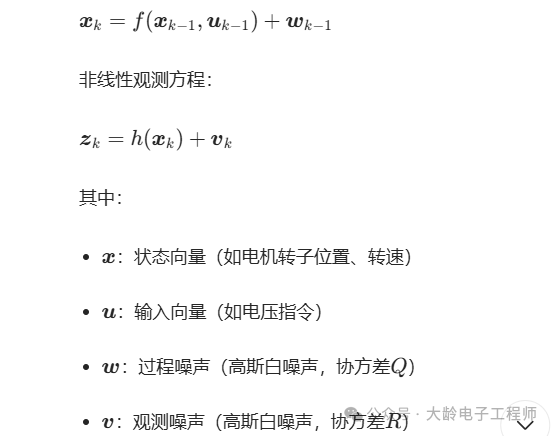


3. C Implementation of EKF
Below is a general EKF framework code (using motor position/speed estimation as an example):
#include <math.h>#include <string.h>// Matrix dimension definitions#define STATE_DIM 2 // State dimension: [theta, omega]#define OBSERVE_DIM 2 // Observation dimension: [I_d, I_q]#define INPUT_DIM 2 // Input dimension: [U_d, U_q]// EKF structuretypedef struct { float x[STATE_DIM]; // State estimate x^+ float P[STATE_DIM][STATE_DIM]; // Covariance matrix P^+ float Q[STATE_DIM][STATE_DIM]; // Process noise covariance float R[OBSERVE_DIM][OBSERVE_DIM]; // Observation noise covariance float F[STATE_DIM][STATE_DIM]; // State Jacobian matrix F float H[OBSERVE_DIM][STATE_DIM]; // Observation Jacobian matrix H float K[STATE_DIM][OBSERVE_DIM]; // Kalman gain K float x_pred[STATE_DIM]; // Predicted state x^- float P_pred[STATE_DIM][STATE_DIM]; // Predicted covariance P^-} EKF_TypeDef;2. Matrix Operation Utility Functions
// Matrix multiplication: C = A*B (m×n)*(n×p) → m×pvoid matrix_mult(float A[][STATE_DIM], float B[][STATE_DIM], float C[][STATE_DIM], int m, int n, int p) { memset(C, 0, sizeof(float)*m*p); for(int i=0; i<m; i++) { for(int j=0; j<p; j++) { for(int k=0; k<n; k++) { C[i][j] += A[i][k] * B[k][j]; } } }}// Matrix transpose: B = A^T (m×n) → n×mvoid matrix_transpose(float A[][STATE_DIM], float B[][STATE_DIM], int m, int n) { for(int i=0; i<m; i++) { for(int j=0; j<n; j++) { B[j][i] = A[i][j]; } }}// 2×2 matrix inversion: B = A^-1void matrix_inv_2x2(float A[2][2], float B[2][2]) { float det = A[0][0]*A[1][1] - A[0][1]*A[1][0]; if(fabs(det) < 1e-6) return; // Singular matrix float inv_det = 1.0f / det; B[0][0] = A[1][1] * inv_det; B[0][1] = -A[0][1] * inv_det; B[1][0] = -A[1][0] * inv_det; B[1][1] = A[0][0] * inv_det;}3. EKF Initialization
void EKF_Init(EKF_TypeDef *ekf) { // Initial state: position 0, speed 0 ekf->x[0] = 0.0f; // theta ekf->x[1] = 0.0f; // omega // Initial covariance: high uncertainty ekf->P[0][0] = 1.0f; ekf->P[0][1] = 0.0f; ekf->P[1][0] = 0.0f; ekf->P[1][1] = 1.0f; // Process noise covariance: adjust based on system characteristics ekf->Q[0][0] = 1e-4f; ekf->Q[0][1] = 0.0f; ekf->Q[1][0] = 0.0f; ekf->Q[1][1] = 1e-3f; // Observation noise covariance: adjust based on current sampling accuracy ekf->R[0][0] = 1e-3f; ekf->R[0][1] = 0.0f; ekf->R[1][0] = 0.0f; ekf->R[1][1] = 1e-3f;}4. Core EKF Computation (Prediction + Update)
// State equation f(x, u): predict next statevoid EKF_State_Model(float x_prev[], float u[], float x_pred[], float Ts) { // theta_pred = theta_prev + omega_prev * Ts x_pred[0] = x_prev[0] + x_prev[1] * Ts; // omega_pred = omega_prev + (Te - TL)/J * Ts (simplified: assume Te is known, TL=0) float Te = 1.0f; // Example: electromagnetic torque (actual calculation needed) float J = 0.01f; // Moment of inertia x_pred[1] = x_prev[1] + (Te / J) * Ts;}// Calculate state Jacobian matrix Fvoid EKF_Calc_F(float x[], float Ts, float F[][STATE_DIM]) { // F = df/dx = [d(theta)/d(theta), d(theta)/d(omega); // d(omega)/d(theta), d(omega)/d(omega)] F[0][0] = 1.0f; F[0][1] = Ts; F[1][0] = 0.0f; F[1][1] = 1.0f; // Simplified model, omega has no partial derivative with respect to theta}// Observation equation h(x, u): predict observation valuesvoid EKF_Observe_Model(float x_pred[], float u[], float z_pred[]) { // Example: PMSM current observation model (simplified) float theta = x_pred[0]; float U_d = u[0], U_q = u[1]; float R = 0.5f; // Stator resistance float L_d = 0.001f, L_q = 0.001f; // Inductance float Ke = 0.1f; // Back EMF coefficient // I_d = (U_d - R*I_d - omega*L_q*I_q)/L_d (actual calculation needs iteration, simplified here) z_pred[0] = (U_d) / (R + L_d / Ts); // I_q = (U_q - R*I_q + omega*L_d*I_d - Ke*omega)/L_q z_pred[1] = (U_q - Ke*x_pred[1]) / (R + L_q / Ts);}// Calculate observation Jacobian matrix Hvoid EKF_Calc_H(float x_pred[], float H[][STATE_DIM]) { // H = dh/dx = [d(I_d)/d(theta), d(I_d)/d(omega); // d(I_q)/d(theta), d(I_q)/d(omega)] H[0][0] = 0.0f; H[0][1] = 0.0f; // I_d has no partial derivative with respect to theta/omega (simplified) H[1][0] = 0.0f; H[1][1] = -0.1f / (0.5f + 0.001f / 1e-4f); // I_q partial derivative with respect to omega}// EKF main function: input u (control), z (observation), Ts (sampling period)void EKF_Update(EKF_TypeDef *ekf, float u[], float z[], float Ts) { // -------------------------- 1. State Prediction -------------------------- EKF_State_Model(ekf->x, u, ekf->x_pred, Ts); // -------------------------- 2. Covariance Prediction ----------------------- EKF_Calc_F(ekf->x, Ts, ekf->F); // Calculate F matrix float F_T[STATE_DIM][STATE_DIM]; matrix_transpose(ekf->F, F_T, STATE_DIM, STATE_DIM); // F^T float F_P[STATE_DIM][STATE_DIM]; matrix_mult(ekf->F, ekf->P, F_P, STATE_DIM, STATE_DIM, STATE_DIM); // F*P matrix_mult(F_P, F_T, ekf->P_pred, STATE_DIM, STATE_DIM, STATE_DIM); // F*P*F^T // Add process noise Q for(int i=0; i<STATE_DIM; i++) { for(int j=0; j<STATE_DIM; j++) { ekf->P_pred[i][j] += ekf->Q[i][j]; } } // -------------------------- 3. Calculate Kalman Gain K -------------------- EKF_Calc_H(ekf->x_pred, ekf->H); // Calculate H matrix float H_T[OBSERVE_DIM][STATE_DIM]; matrix_transpose(ekf->H, H_T, OBSERVE_DIM, STATE_DIM); // H^T float H_P[OBSERVE_DIM][STATE_DIM]; matrix_mult(ekf->H, ekf->P_pred, H_P, OBSERVE_DIM, STATE_DIM, STATE_DIM); // H*P^- float H_P_Ht[OBSERVE_DIM][OBSERVE_DIM]; matrix_mult(H_P, H_T, H_P_Ht, OBSERVE_DIM, STATE_DIM, OBSERVE_DIM); // H*P^-*H^T // Add observation noise R for(int i=0; i<OBSERVE_DIM; i++) { for(int j=0; j<OBSERVE_DIM; j++) { H_P_Ht[i][j] += ekf->R[i][j]; } } // Inversion: (H*P^-*H^T + R)^-1 float H_P_Ht_inv[OBSERVE_DIM][OBSERVE_DIM]; matrix_inv_2x2(H_P_Ht, H_P_Ht_inv); // K = P^- * H^T * (H*P^-*H^T + R)^-1 float P_Ht[STATE_DIM][OBSERVE_DIM]; matrix_mult(ekf->P_pred, H_T, P_Ht, STATE_DIM, STATE_DIM, OBSERVE_DIM); matrix_mult(P_Ht, H_P_Ht_inv, ekf->K, STATE_DIM, OBSERVE_DIM, OBSERVE_DIM); // -------------------------- 4. State Update -------------------------- float z_pred[OBSERVE_DIM]; EKF_Observe_Model(ekf->x_pred, u, z_pred); // Predict observation values float z_error[OBSERVE_DIM]; for(int i=0; i<OBSERVE_DIM; i++) { z_error[i] = z[i] - z_pred[i]; // Observation residual } // x^+ = x^- + K*(z - h(x^-)) for(int i=0; i<STATE_DIM; i++) { ekf->x[i] = ekf->x_pred[i]; for(int j=0; j<OBSERVE_DIM; j++) { ekf->x[i] += ekf->K[i][j] * z_error[j]; } } // -------------------------- 5. Covariance Update ------------------------ float I_KH[STATE_DIM][STATE_DIM]; float K_H[STATE_DIM][STATE_DIM]; matrix_mult(ekf->K, ekf->H, K_H, STATE_DIM, OBSERVE_DIM, STATE_DIM); // I_KH = I - K*H for(int i=0; i<STATE_DIM; i++) { for(int j=0; j<STATE_DIM; j++) { I_KH[i][j] = (i==j ? 1.0f : 0.0f) - K_H[i][j]; } } // P^+ = (I - K*H)*P^- matrix_mult(I_KH, ekf->P_pred, ekf->P, STATE_DIM, STATE_DIM, STATE_DIM);}5. Example of EKF Usage
int main() { EKF_TypeDef ekf; EKF_Init(&ekf); float Ts = 1e-4f; // 100us sampling period float u[INPUT_DIM] = {0.0f, 1.0f}; // U_d=0, U_q=1V float z[OBSERVE_DIM] = {0.1f, 2.0f}; // Measured I_d, I_q while(1) { EKF_Update(&ekf, u, z, Ts); // EKF iteration float theta_est = ekf->x[0]; // Estimated position float omega_est = ekf->x[1]; // Estimated speed }}6. Key Considerations
- Accuracy of Jacobian Matrix: EKF relies on first-order linearization, and the accuracy of the Jacobian matrix directly affects the filtering performance, requiring strict derivation.
- Tuning of Noise Covariance Q/R
- Increasing Q → faster tracking, but weaker noise suppression;
- Increasing R → trust predictions, distrust observations; conversely, trust observations.
7. Extended Applications
EKF is widely used in:
- Sensorless FOC of motors (position/speed estimation);
- Drone attitude estimation (IMU+GPS fusion);
- Target tracking (radar/vision fusion).
With the above code framework, EKF can be quickly implemented and adapted to specific nonlinear systems, with the core being to modify the state equations, observation equations, and Jacobian matrices according to the actual scenario.