Welcome to the Battery Perspective!
In the overview of SOC (State of Charge) estimation methods, various SOC estimation techniques are introduced, and we will provide corresponding analyses and application introductions for each method. Previously, we discussed the Ampere-hour integration method (SOC estimation – Sources of error and impact of Ampere-hour integration), and here we will introduce the OCV method.
The OCV method primarily relies on the monotonicity of the OCV-SOC curve for tabulation. The battery voltage (note that this refers to terminal voltage) is very easy to collect and must be obtained; theoretically, once the voltage is acquired, the SOC can be determined immediately.
In practice, there are two issues that need to be addressed: first, how to obtain the OCV-SOC curve, and second, how to relate the OCV to the measured battery voltage.
The common methods for testing OCV are the small current method and the capacity increment method. Figure 1 shows the OCV curves of the same battery tested at different temperatures using a small current (0.05C).
There are several issues here: 1. OCV is affected by temperature, leading to different SOCs corresponding to the same OCV at different temperatures; 2. Charging OCV and discharging OCV differ, resulting in different SOCs corresponding to the same OCV during charging and discharging; 3. The capacity during charging and discharging is different, leading to different SOCs corresponding to the same OCV during charging and discharging; 4. During use, there is an overpotential between the dynamic terminal voltage and OCV, making direct use impossible.
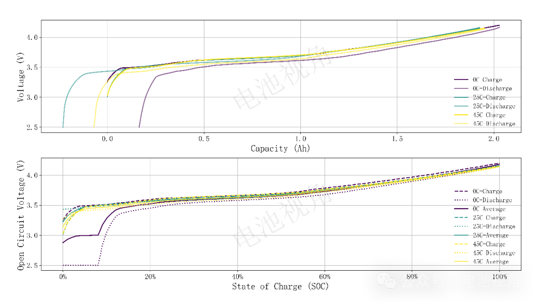
Figure 1. OCV curves of charging and discharging at different temperatures obtained using the small current method.
The temperature issue can be alleviated by testing data at different temperature windows. For the selection of charging and discharging OCV, we first consider using the average OCV (forcing the capacities of charging and discharging to normalize to the 0-1 range), as shown in Figure 1 (the lower figure), but the results are clearly not ideal, especially when the charging and discharging capacities are inconsistent, leading to significant deformation of the OCV curve, making it difficult to use.
Figure 2 shows the OCV curves tested using the capacity increment method. The testing process involves current pulse – rest – current pulse – rest, until the specified voltage is reached, and then the voltage-capacity curve is obtained from the end of the rest period, as shown in Figure 3. From Figure 3, it can be seen that the OCV tested using the capacity increment method during charging or discharging in a ternary system overlaps quite well, providing uniqueness for our selection.
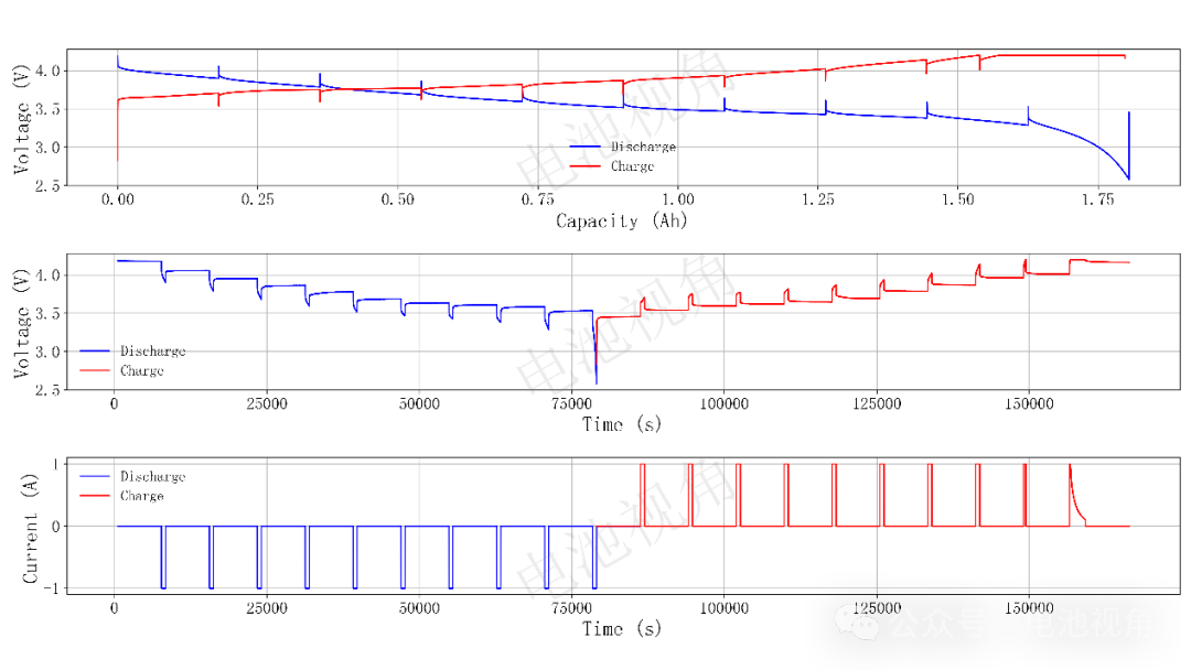
Figure 2. OCV curves during the charging and discharging process tested using the capacity increment method.
In fact, this uniqueness is also relative, as the two do not completely overlap. The bottom figure in Figure 3 shows the SOC corresponding to the same OCV during charging and discharging and their differences, indicating that errors clearly exist.
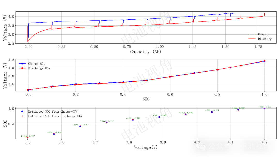
Figure 3. OCV curves tested using the capacity increment method.
Additionally, the capacity increment method has another issue: during the pulse-rest-pulse-rest testing process, how long should the rest period be? The OCV obtained with different rest times varies. This is because during the rest period, there is a process of Ohmic voltage drop and concentration gradient elimination; different rest times lead to different degrees of concentration gradient elimination, resulting in different OCVs, which inevitably leads to different SOCs obtained through interpolation.
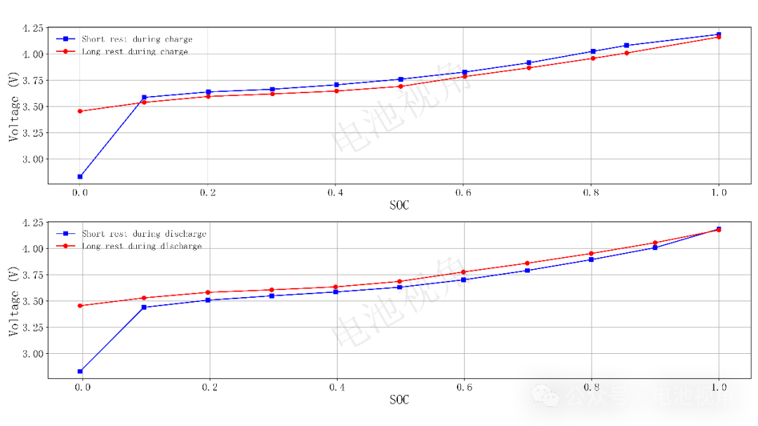
Figure 4. OCV-SOC curves at different rest times during the capacity increment method testing.
Even if we stipulate: 1. All reference OCV curve tests have a sufficiently long rest time; 2. Reference charging OCV curve during charging, reference discharging OCV curve during discharging; 3. The temperature during SOC estimation is consistent with the temperature during OCV testing, the estimation of SOC will still be affected by polarization.
To address the impact of polarization, voltage compensation is often required. For Ohmic voltage drop, it is sufficient to subtract the product of current and Ohmic resistance from the charging voltage or add it to the discharging voltage. The figure below shows the results of obtaining OCV by compensating for Ohmic voltage drop in the short time after the pulse starts (considered short enough that only Ohmic voltage drop is manifested). It is evident that after compensation, an accurate OCV can almost be obtained, which is very beneficial for estimating SOC using the OCV method.
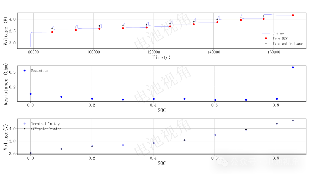
Figure 5. Eliminating Ohmic voltage drop through voltage compensation.
However, after the pulse starts, reaction polarization and concentration polarization appear one after another, making voltage compensation very complex. We will introduce compensation methods later.