Click the blue text

Follow us

Pengye Jiatu Technology
September 19, 2025
Issue 4: In-Depth Analysis of the 2025 FPGA Competition Topic 2 Analysis
Hello everyone, we are Pengye Jiatu Technology~ In this issue, we will bring you an analysis of the 2025 FPGA Innovation Design Competition Topic 2, with over 7000 words of detailed analysis, packed with valuable information. If you stick around until the end, it will definitely help you! Below is our original analysis video, and you can also follow our Bilibili account:RyanFPGA to watch it simultaneously!

Analysis Video

Followed Follow Replay Share Like <!– –> Watch morePengye Jiatu Technology
0/0
00:00/12:26Progress bar, 0 percentPlay00:00/12:2612:26Full screen Playing at speed 0.5x 0.75x 1.0x 1.5x 2.0x Ultra clear Smooth
Continue watching
In-Depth Analysis of the 2025 FPGA Competition Topic 2: How FPGA Solves the Challenges of Real-Time Performance and Accuracy in Industrial Inspection
Original, In-Depth Analysis of the 2025 FPGA Competition Topic 2: How FPGA Solves the Challenges of Real-Time Performance and Accuracy in Industrial InspectionPengye Jiatu TechnologyAdded to Top StoriesEnter comment Video Details
That’s all for this issue’s analysis video of Topic 2, next we present a super detailed text analysis that will be clearer and easier to understand. First, let’s look at the design requirements of this topic!
(For the complete learning route and related materials, please add WeChat at the end of the article to obtain)

1. Background Introduction
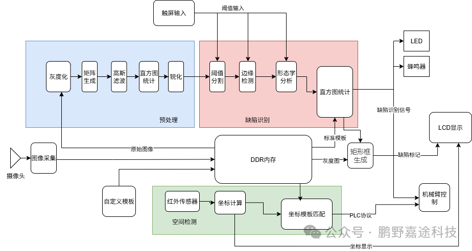
FPGA has a wide range of applications in the field of intelligent manufacturing, which can be used to accelerate image processing algorithms and sensor data processing, such as edge detection, filtering, binarization, and laser radar positioning. Due to its parallel processing capability, low latency, and hardware customizability, it is an ideal platform for industrial defect detection and spatial positioning detection.
In industrial production, yield is a key indicator, so detecting defective and substandard products is an indispensable and crucial step. Good defect detection can reduce production costs, minimize losses from returns, and enhance product reputation. Using FPGA to accelerate image processing algorithms can improve detection efficiency and accuracy; in spatial position detection, FPGA can accelerate sensor data processing. If data is transmitted to a computer for processing, it will introduce significant latency and energy consumption, while using FPGA can achieve real-time data processing and analysis, greatly improving detection efficiency and accuracy, making it a key technology for ensuring product quality and production efficiency. Therefore, participants need to develop a multifunctional detection system based on FPGA for industrial manufacturing, achieving defect identification, spatial positioning, and automated feedback control.

2. Hardware Recommendations
Participants in this competition should use the specified Ziguang Tongchuang FPGA development platforms, including the following models: Pangu 50, Pangu 676 series development boards, PGX-NANO, RK3568_MES2L50H, with a recommendation to use the PG2L100H board from the 676 series. Onboard ADC, DAC, LCD, buttons, LEDs, and expandable SPI/I2C interface devices (such as Flash, SD cards) are allowed. Additionally, a camera necessary for functionality should be implemented.

3. Competition Requirements
1

Core Functional Modules
Industrial Defect Detection
Image Acquisition and Preprocessing: Use FPGA to drive industrial cameras to acquire product images, completing grayscale conversion, noise reduction (median filtering), edge enhancement, and other preprocessing in real-time (during the competition, images can also be tested through HDMI or other interfaces as input images; image acquisition will not be scored).
Defect Recognition Algorithm: Design image processing algorithms based on FPGA parallel computing (such as template matching, threshold segmentation, morphological analysis) to detect and mark defect areas for typical scenarios such as scratches on metal surfaces and PCB welding defects; support custom defect templates, with parameters uploaded via buttons or touch screens.
Detection Accuracy: The minimum defect detection size is less than 10cm*10cm, and the higher the detection accuracy, the higher the score.
Spatial Position Detection
Multi-Sensor Fusion Positioning: Combine laser radar (simulated distance measurement), infrared sensor arrays, etc., to achieve two-dimensional or three-dimensional spatial position detection of workpieces, with FPGA processing sensor data in real-time to calculate workpiece coordinates (X/Y/Z axes) and attitude angles (pitch/yaw/roll), with higher positioning accuracy being better.
2

System Interaction and Feedback
Human-Machine Interaction Interface: Display detection results, real-time images, and position coordinates through a touch screen or LCD; support parameter settings (such as detection thresholds, sensor calibration).
Sound and Light Alarm and Control Output: Trigger a buzzer and LED flashing alarm when defects or position deviations exceed limits.
Output control signals through GPIO (such as PLC interface protocol) to link robotic arms to remove defective products or adjust equipment parameters.
3

Performance Optimization and FPGA Advantages
Real-Time Performance: The total delay for defect detection and position calculation should be as low as possible; the lower the delay, the higher the score, aiming to meet the high-speed detection requirements of industrial assembly lines.
Resource Customization: Utilize FPGA’s parallel processing capabilities to hardware accelerate image algorithms and sensor data processing modules, improving performance compared to ARM platforms.
Scalability: Reserve SPI and I2C interfaces to support external sensors (such as pressure sensors, RFID).
Scalability: In industrial production, there are various types of defects. For example, to detect scratches on metal surfaces, capture images with a camera and begin preprocessing; during the defect recognition phase, detect the edge parts and extract features; when a non-compliance is detected, use a rectangle generator to frame the defect area and output it to the display.
4. Function Implementation
01
Industrial Defect Detection
1.1

Image Acquisition
Use FPGA to drive industrial cameras to capture real-time images; the method of image acquisition is not limited, and any method can be chosen based on actual needs.
01
OV5640 Camera Acquisition
The OV5640 camera supports outputting images with a maximum of 5 million pixels (2592×1944 resolution), using DVP interface, and supports data formats of YUV422, RGB565, and JPEG. The smaller data volume allows for low-latency transmission, but the color accuracy is relatively low.
Image preprocessing includes grayscale conversion, binarization, filtering, image enhancement, etc., which can simplify input image data, filter noise, and enhance features, outputting smaller data volume and smoother grayscale data stored in DDR, facilitating faster processing and more accurate identification by defect recognition algorithms, improving detection real-time performance and accuracy.
1.2

Grayscale Conversion
01
Grayscale Conversion
Grayscale conversion is the process of converting RGB to YUV format. The YUV (YCbCr) format is used to describe the saturation and hue of images, where Y represents brightness, and U and V represent chrominance. This can simplify image information, remove redundant information, and reduce the data volume required for calculations, enhancing computational efficiency, and is the foundation of all image processing. YCbCr is derived from YUV, and in general, the two are equivalent, with Y still representing brightness, Cb representing the blue component, and Cr representing the red component.
A well-known psychological formula for color grayscale conversion comes from the following RGB888 to YCbCr formula:
Y = 0.299R +0.587G + 0.114B
Cb = 0.568(B-Y) + 128 = -0.172R-0.339G + 0.511B + 128
Cr = 0.713(R-Y) + 128 = 0.511R-0.428G -0.083B + 128
The output grayscale image compared to the original image is shown below:


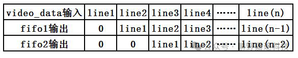
Matrix Generation: In digital image processing, some algorithms require calculations based on each pixel and its surrounding pixel data within a certain range. In the case of image data being input row-wise, to obtain a 3X3 image matrix, data from three rows of the image must be output simultaneously, implemented using a line buffer + shift register structure.
The output result is:
02
BinaryizationGreat Heat
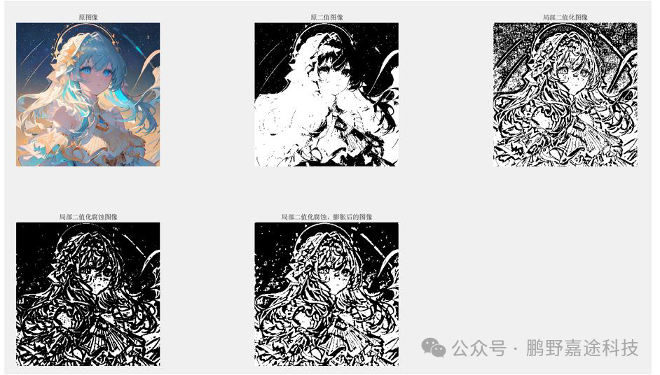
Set the grayscale value (8bit) of each pixel point in the image to 0 or 255, resulting in a black-and-white effect. If the focus is not on color and image details but rather on contours, edges, or recognizing certain features, binaryization can simplify the data.
Binaryization can be divided into global binaryization and local binaryization. Global binaryization selects a number as a threshold from 0 to 255, while local binaryization generates a 3X3 image matrix and calculates the average of the grayscale values in each 3×3 window, using the average as the threshold.

03
Mean Filtering
Mean filtering replaces the value of a pixel with the average value of its neighboring pixels. The principle is to use a window (such as 3×3 or 5×5) to cover the target pixel and its neighbors, calculate the average of all pixel values in that area, and replace the center pixel’s value with this average, then slide the window to each pixel position in the image and repeat the operation. The mean filtering algorithm is simple to implement, has a small computational load, and can effectively smooth images and reduce noise, but it can also blur image details and edges, so it is best not to choose this method in industrial detection scenarios where edge details need to be preserved.
04
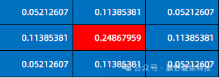
Median Filtering
The color gradient of an image is displayed through linear changes of the three RGB colors. If the value of a certain point in an image differs too much from the surrounding values, it can be identified as noise. The median filtering algorithm takes the median value of the data surrounding this point within a window, helping to filter out salt-and-pepper noise in images, suitable for processing isolated noise points.
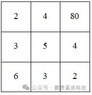
As shown in the above image, there is a 3×3 YUV image data matrix, where the data 80 has a significant color value difference from surrounding points. Reflected in the image, it should be a noise point that is brighter than surrounding values. Using the median filtering algorithm, the following processing is performed on the original data matrix:
First, perform a sorting algorithm. The first step is to sort each row’s elements from largest to smallest to output a matrix.
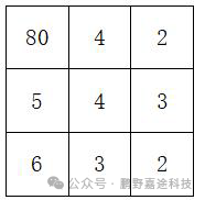
Second, sort the largest, middle, and smallest elements from each row to obtain:
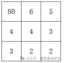
Third, sort the largest (top right 5), middle (center 4), and smallest (bottom left 3) to take the middle value 4 as the median. For each pixel, perform a row field scan, and when a noise point is scanned, that point will not be output, achieving noise filtering.
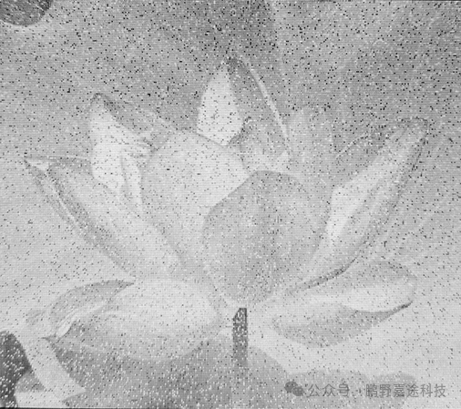
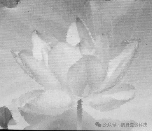
The comparison before and after filtering is as follows:
05
Gaussian Filtering
Gaussian noise refers to a type of noise whose probability density function follows a Gaussian distribution (i.e., normal distribution). If the amplitude distribution of a noise follows a Gaussian distribution and the power spectral density is uniformly distributed, it is called Gaussian white noise. In industrial scenarios, environmental temperature, poor lighting, and other factors may cause the signals captured by cameras to introduce Gaussian noise.
The two-dimensional Gaussian probability density distribution function is:
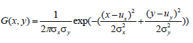
Gaussian filtering is the process of performing weighted averaging on the entire image through convolution operations, with the convolution kernel as a reference:
Gaussian filtering minimizes the impact of noise as much as possible, but does not consider the coherence of noise, and does not protect edges well, easily producing black edges.
06
bilateral filtering algorithm
The bilateral filtering algorithm simultaneously considers the influence of pixel spatial distance and pixel similarity (the brightness difference between surrounding pixels and the center pixel) on the weight, effectively reducing noise while preserving image edge effects. Multiply the pixel weight and spatial weight, then substitute into the matrix to form a bilateral filtering convolution kernel to perform operations similar to Gaussian filtering.
07
Edge Enhancement
The Laplacian operator is a second-order differential operator that produces a strong response in areas of rapid change in image grayscale (high-frequency parts), which are precisely the edges. After processing, it can sharpen the image. The Laplacian operator is implemented through convolution operations, with the convolution kernel as follows:
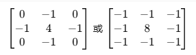
After convolution calculation, the edges can be enhanced by overlaying them with the original image.
08
Image Enhancement
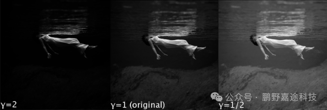
Histogram equalization is a common image enhancement method that can make the grayscale of an image as evenly distributed as possible, resulting in higher contrast, making weak scratches on metal surfaces more visible against the background.
In industrial inspection, due to lighting effects, even defect-free workpieces may exhibit local brightness differences, leading to misjudgments. To reduce local shadows and lighting variations in images, gamma correction should be applied to adjust the overall brightness of the image.
Below is a comparison of outputs with different gamma values:
1.3

Defect Recognition Algorithm
For typical scenarios such as scratches on metal surfaces and PCB welding defects, design image processing algorithms based on FPGA parallel computing (such as template matching, threshold segmentation, morphological analysis) to detect and mark defect areas; support custom defect templates, with parameters uploaded via buttons or touch screens. Detection accuracy: the minimum defect detection size is less than 10cm*10cm, the smaller the size, the higher the accuracy, and detection accuracy and precision are the main indicators.
Threshold Segmentation
Use Otsu’s algorithm (i.e., Otsu’s method – maximum inter-class variance method) for threshold segmentation, automatically selecting an appropriate threshold by maximizing the inter-class variance based on the histogram of the image’s grayscale distribution, separating the background from the defect area. The threshold can be further optimized based on preset defect sizes and shape features. Once the threshold is confirmed, binarization or feature extraction can be performed.
The threshold T divides the pixel color values into two categories, with the probability of foreground color being p1 for values less than or equal to the threshold, and p2 for values greater than the threshold, with color means m1 and m2, and the overall pixel mean being mG. The inter-class variance is:
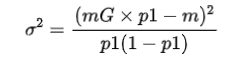
Find a grayscale value m that maximizes this variance, which will be the threshold T.
Note: When the area of the target and background is not significantly different, effective image segmentation can be achieved; when the area of the target and background differs greatly, the histogram may not show a clear bimodal distribution, resulting in poor segmentation, or when there is a large overlap in grayscale between the target and background, accurate separation cannot be achieved.
Edge Detection
Edge detection calculations in image processing generally use the Sobel operator, which is performed on the basis of grayscale conversion. Edge detection is also very sensitive to noise, so Gaussian filtering should be applied for noise reduction first. The Sobel operator is a discrete first-order differential operator, and its principle is based on image convolution to detect edges in the horizontal and vertical directions.
Canny edge detection is an upgraded version of Sobel in industrial vision, which performs non-maximum suppression and double threshold detection based on Sobel, depicting edges more accurately.
Morphological Analysis
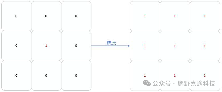
Morphological analysis is a set-theoretic image processing method that includes operations such as erosion, dilation, opening, and closing. Erosion and dilation are applied to binary images, where erosion can eliminate some rough edges or isolated noise points, smoothing certain boundaries in the image.

The effect of dilation is to fill certain voids, connect broken scratches, and expand certain parts to connect boundaries, etc.
The combined use of erosion and dilation is opening and closing operations, where opening (erosion followed by dilation) is used to remove noise points and small protrusions in the image, and closing (dilation followed by erosion) is used to fill small holes and repair small gaps in object edges. In defect detection, morphological processing can be used to optimize the results after threshold segmentation or edge detection, removing some false defects or repairing incomplete boundaries of defect areas.
However, this method can also cause issues such as excessive erosion and dilation. If a threshold is introduced, erosion and dilation operations can be performed only when the sum of pixel values in the matrix exceeds the threshold, allowing for adjustable intensity of erosion and dilation.
Template Matching
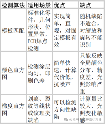
The core of the template matching algorithm is to calculate the similarity between image blocks and standard templates, using feature vector matching or common correlation coefficients or mean square errors to measure similarity. The higher the similarity, the closer it is to the standard template; conversely, it indicates a defect. This algorithm has relatively high precision and is suitable for detecting irregular surface defects or geometric shape defects of known shapes under fixed posture and position, such as parts made using molds, PCB solder joint detection, printed text, etc. However, it is not sensitive to shapes outside the template or defects that have been rotated or scaled, making it prone to missing detections.
There are several methods to achieve this:Normalized cross-correlation method, minimum error method, feature vector matching method.
Gradient Histogram Statistics
Color Histogram can quickly describe the statistical information of the overall pixel value distribution of an image, showing the number of pixels within a certain pixel value range. It is suitable for defect types with color differences in color blocks. Its algorithm is simple and fast, requiring minimal processing, and has strong noise resistance, but it can only reflect the global color distribution and cannot describe local features of the image, resulting in lower precision.
For defect types that are random in shape, position, and direction, such as metal scratches,Gradient Direction Histogram Statistics (HOG) can effectively extract local shape and texture features from images, capturing more complex defect types, suitable for defects with significant morphological variations. However, HOG has a larger computational load than color histograms and is sensitive to rotation and scale changes.
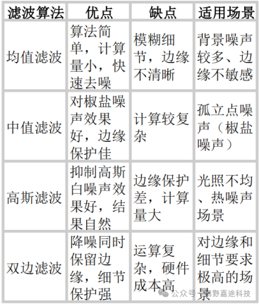
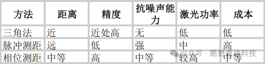
Comparison of Various Defect Recognition Algorithms
Detection Accuracy
Detection Accuracy: The minimum defect detection size is less than 10cm*10cm, and the higher the detection accuracy, the higher the score.
To improve accuracy and detection precision, there are various methods: during the image acquisition phase, higher resolution can be used. In the preprocessing phase, better algorithms can be used for noise reduction; bilateral filtering can reduce noise while preserving edge details, followed by using the Laplacian operator for edge enhancement and gamma correction algorithms for image sharpening, making defects more prominent.
In feature extraction and matching, multi-scale detection can be increased to extract features at different scales, detecting defects of various sizes; during detection, images can be divided into several small blocks for local detection, increasing precision.
In defect recognition algorithms, using the Canny operator for edge detection can output higher precision edge data; or directly incorporating machine learning: introducing simple classifiers (such as SVM or decision trees) to classify features, improving detection capabilities in complex scenarios.
In terms of data, increasing the diversity of normal templates can reduce false positives; generating more defect samples through rotation, scaling, flipping, etc., can enhance the robustness of the algorithm. Through the human-machine interaction interface, real-time monitoring of detection results is supported, allowing for manual adjustment of detection parameters to ensure detection accuracy.
1.4

Spatial Position Detection
Multi-Sensor Fusion Positioning
Combine laser radar (simulated distance measurement), infrared sensor arrays, etc., to achieve two-dimensional or three-dimensional spatial position detection of workpieces.
Common methods for laser radar ranging include triangulation, pulse ranging, and phase ranging. Triangulation has the highest precision at close distances, suitable for near-range detection, but has almost no anti-interference capability; even a slight angle deviation can significantly affect measurement results.
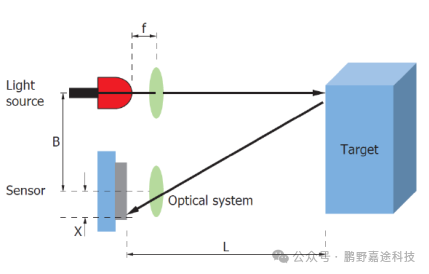
Triangulation Ranging
Triangulation laser radar determines distance L = f(L+x)/x based on the imaging position of the camera’s light spot.
Pulse Ranging
Pulse ranging is the simplest method, calculating distance based on the time it takes for the laser to reflect off the target surface and return, with the distance formula being L=ct/2. It is suitable for medium to long-distance measurements.
Phase Ranging
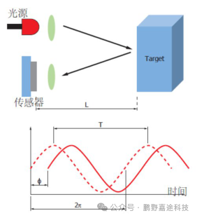
Phase ranging involves modulating the laser signal before emission and calculating distance based on the phase difference between the received and emitted signals, achieving millimeter to micrometer level precision, suitable for medium to short-distance measurements. Its calculation formula is

Distance can be determined without measuring time and frequency, only requiring knowledge of wavelength and phase difference.
When testing the two-dimensional coordinates of a workpiece, the camera should be aligned with the workpiece, deriving the XY pixel coordinate values based on the edge pixel positions, and then calculating the spatial coordinates using distance and camera parameters.
Binocular Ranging
The principle of binocular ranging is to deduce the depth value of the scene through the parallax of two camera images, similar to triangulation. Corresponding points of the same object are found in the left and right images, and the parallax is calculated as the horizontal position difference between the left and right camera imaging points. The distance can then be calculated using focal length, pixel difference, and the baseline length of the binocular camera.
Infrared Sensor Array
The infrared sensor array consists of a linear array or two-dimensional matrix of multiple infrared emitters and receivers, with each detector corresponding to a spatial sampling point; its working principle is that when an object enters the detection range of the array, it blocks the emitted infrared light, changing the intensity of the infrared signals received by certain points, thus identifying the object’s position.
The benefit of multi-sensor fusion is that different sensors complement each other, avoiding blind spots and errors caused by a single sensor, thus ensuring positioning accuracy and stability. Therefore, in industrial detection, infrared arrays are often used as a rough positioning method, quickly determining the approximate location of an object, and then using high-resolution cameras for detailed detection to obtain pixel coordinates.
Sensor Data Processing
FPGA processes sensor data in real-time, calculating workpiece coordinates (X/Y/Z axes) and attitude angles (pitch/yaw/roll), with higher positioning accuracy being better.
The relationship between pixel coordinates and world coordinates is shown in the figure below:
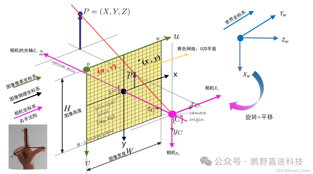
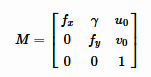
In sensor coordinate calculations, intrinsic parameters describe the internal properties of the camera, including focal length, principal point coordinates, distortion coefficients, etc., while extrinsic parameters mainly describe the spatial position and attitude relationship between the sensor coordinate system and the world coordinate system.
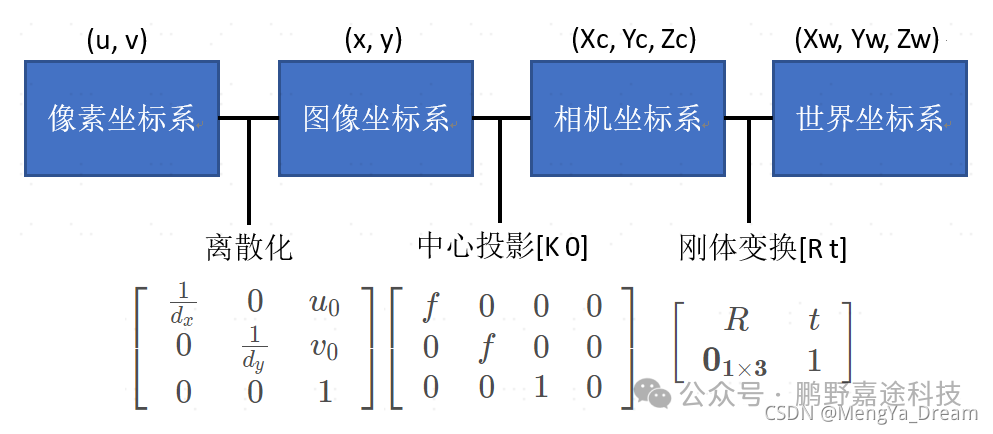
To convert feature point pixel coordinates to spatial coordinates, the camera’s intrinsic parameters must first be determined.
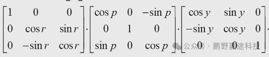
The following figure shows the extrinsic parameter matrix, where R is the rotation matrix calculated using attitude angles, and t is the translation vector.

The attitude angle measurement is achieved using an IMU, i.e., an Inertial Measurement Unit, where the xyz axes correspond to roll, pitch, and yaw angles:
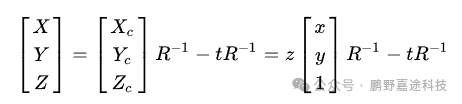
Finally, the world coordinates are deduced through inverse calculation.
02
System Interaction and Feedback

2.1

Human-Machine Interaction Interface
Display detection results, real-time images, and position coordinates through a touch screen or LCD; support parameter settings (such as detection thresholds, sensor calibration).
Results and defect markings are displayed through a text display module and rectangle generation module, with threshold values input via the touch screen written into registers. Common touch screens include resistive screens (using AD converters), capacitive screens (using I2C interfaces), or using Raspberry Pi as the host computer.
2.2

Sound and Light Alarm
Trigger a buzzer and LED flashing alarm when defects or position deviations exceed limits.
Whenever a defect is detected, or the coordinates of the workpiece being tested deviate from the standard coordinates by a certain threshold, an enable signal is output to the LED and buzzer.
2.3

GPIO Control Output
Output control signals through GPIO (such as PLC interface protocol) to link robotic arms to remove defective products or adjust equipment parameters.
When a defect is detected, the coordinates of the workpiece are locked based on the detected spatial coordinates, outputting control signals to the robotic arm to push the defective products away.
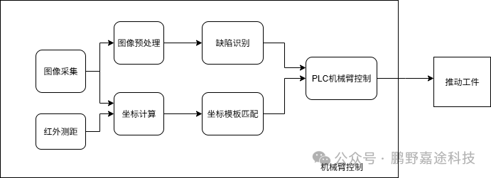
The robotic arm does not need too many degrees of freedom; it only needs to perform simple push and pull actions.
Generally, in stepper servo control, the PLC protocol uses pulse frequency to control motor output power to change speed, using pulse count to control the total number of rotations of the servo motor, thus controlling the angle of the robotic arm and generating control signals.
#1
Real-Time Performance
The total delay for defect detection and position calculation should be as low as possible; the lower the delay, the higher the score, aiming to meet the high-speed detection requirements of industrial assembly lines. To enhance real-time performance, choose a reasonable clock frequency, use a pipelined structure to optimize critical paths, and improve real-time performance; more BRAM can be used to cache data, avoiding frequent access to DDR.
#2
Resource Customization
Utilize FPGA’s parallel processing capabilities to hardware accelerate image algorithms and sensor data processing modules, improving performance compared to ARM platforms.
Implement multi-channel parallel computing, and for complex operations like quantization of directional vectors, try to use LUT lookup tables instead, approximating square root operations of gradient magnitudes. Compared to software implementations, FPGA can reduce processing delays from milliseconds to microseconds, achieving acceleration factors of 10-100 times, especially in high-speed assembly lines in edge computing.
#3
Scalability
Reserve SPI and I2C interfaces to support external sensors (such as pressure sensors, RFID). The I2C interface is used to configure OV5640 registers.
(For the complete learning route and related materials, please add WeChat at the end of the article to obtain)
References
1. Parallel Processing Analysis of Grayscale Image Template Matching Based on FPGA – Computer Application Technology Thesis.docx
(https://max.book118.com/html/2019/0110/8105100140002000.shtm)
2. (PDF) Scratch Detector – A FPGA Based System for Scratch Detection in Industrial Picture Development.(https://www.researchgate.net/publication/221188895_Scratch_Detector_-_A_FPGA_Based_System_for_Scratch_Detection_in_Industrial_Picture_Development)
3. A new lightweight deep neural network for surface scratch detection | The International Journal of Advanced Manufacturing Technology(https://link.springer.com/article/10.1007/s00170-022-10335-8?utm_source=chatgpt.com)
4. Li Liang, Li Dong. A Method for Real-Time Histogram Equalization Based on FPGA[J]. Automation Applications, 2015, 000(10):21-23,35
5. OTSU Algorithm (Otsu’s Method – Maximum Inter-Class Variance Method) Principle and Implementation – CSDN Blog
(https://blog.csdn.net/weixin_40647819/article/details/90179953)
6. Image Segmentation – Using Gradient Algorithm to Improve Global Threshold Setting – Code Pioneer Network(https://www.codeleading.com/article/62362083223/)
7. Image Experiment Guide Manual_Pangu 676 Series 100Pro+ Development Board Tutorial 3
8. [Ziguang Tongchuang FPGA Image Video Tutorial][Based on Pangu 676 Development Board] Bilibili_bilibili(https://www.bilibili.com/video/BV1wYo9YgEJe?spm_id_from=333.788.videopod.sections&vd_source=13c8ce0d9f9b2bcd1effd391a04d4dba)
9. Chen Mingming, Zhu Yongxin, Tian Li, et al. Design of a Real-Time Binocular Ranging Algorithm Based on FPGA[J]. Microelectronics and Computers, 2018, 35(10):5. DOI:CNKI:SUN:WXYJ.0.2018-10-013.
10. FPGA Real-Time Processing Based Binocular Ranging System.pdf – Original Power Document(https://max.book118.com/html/2023/0314/6000234143005101.shtm?from=search&index=2)
11. Coordinate Transformation: The Journey from Image Coordinates to World Coordinates – Zhihu(https://zhuanlan.zhihu.com/p/666365279)
12. Basics of FPGA Image Processing – Histogram Equalization_fpga Histogram Equalization – CSDN Blog(https://blog.csdn.net/qq_41332806/article/details/107213173)
13. [Ziguang Tongchuang FPGA Image Video Tutorial][Based on Pangu 676 Development Board] Character Overlay Code Explanation_Bilibili_bilibili(https://www.bilibili.com/video/BV1cCZnY7E5J/?spm_id_from=333.1387.upload.video_card.click)
14. Logic Z1 Development Board Video Tutorial Episode 1_Bilibili_bilibili(https://www.bilibili.com/video/BV16PQPY7EAr/?spm_id_from=333.1387.upload.video_card.click)
15. Fast Template Matching Algorithm for Multiple Targets and Angles (Based on NCC, Effectively Approaching Halcon)_Pyramid Downsampling Initially Determines Template Matching Angle Range – CSDN Blog(https://blog.csdn.net/weixin_39450742/article/details/118600464)
16. Application of Grayscale Histogram Feature Recognition for Wood Surface Knot Defects(https://www.researching.cn/ArticlePdf/m00002/2015/52/3/031501.pdf)

Follow us to learn more about FPGA knowledge
Video updates are synchronized on our Bilibili account
Bilibili account: RyanFPGA
If you want to get more competition support content, please scan the QR code below to add us on WeChat for further communication!
Like