Introduction

In scientific plotting, it is essential to be both rigorous and visually appealing— especially when visualizing complex scalar fields, topological structures, and field theories. When creating plots for “vortices”, “topological defects”, and “phase fields”, we often encounter the following issues:

• The data is excellent, but the resulting plot is “not sophisticated enough”.

• The surface plot looks rough, gray, and opaque.

• Adjusting the colormap, lighting, and transparency to achieve a state that is “both informative and visually appealing” is challenging.

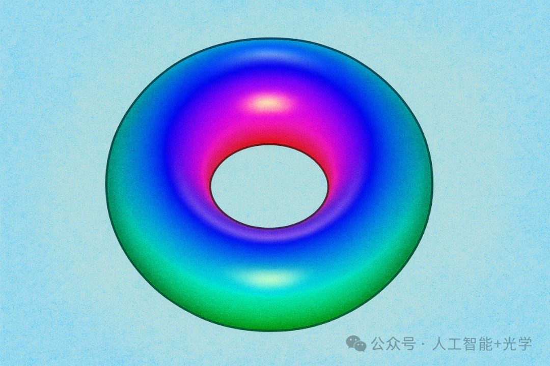
Therefore, in this issue, we will learn about scientific plotting solutions—using Python & MATLAB to create “aesthetically pleasing scalar topological vortex surface plots” (Scalar Topological Vortex Surface). Without further ado, let’s get into the details.

🌄 MATLAB for Scalar Topological Vortex Plotting

    clc    clear all;     close all;       % Initialize window    figure('Color', 'w', 'Position', [100, 100, 800, 600]);    hold on;    axis equal;    axis off;    %% 1. Generate toroidal geometry data    % R: Major radius (distance from the center of the torus to the center of the tube)    % r: Minor radius (tube radius)    R = 4;     r = 1.8;     % Use a higher grid for smoother gradients    num_pts = 200;    [theta, phi] = meshgrid(linspace(0, 2*pi, num_pts), linspace(0, 2*pi, num_pts));    % Toroidal parametric equations    X = (R + r .* cos(phi)) .* cos(theta);    Y = (R + r .* cos(phi)) .* sin(theta);    Z = r .* sin(phi);    %% 2. Define color mapping    phase_shift = 2.5;     C = mod(phi + phase_shift, 2*pi);     %% 3. Plot surface    h = surf(X, Y, Z, C);    %% 4. Visual enhancement    colormap(hsv);     shading interp;     % 4.2 Material settings     material shiny; % Set to shiny material    set(h, ...        'AmbientStrength', 0.5, ...  % Ambient light intensity        'DiffuseStrength', 0.6, ...  % Diffuse light intensity        'SpecularStrength', 0.8, ... % Specular reflection (highlight) intensity, higher values make it brighter        'SpecularExponent', 15);     % Highlight range, larger values make the highlight smaller and sharper    % 4.3 Light settings    light('Position', [0, -10, 10], 'Style', 'local'); % Main light source    light('Position', [0, 10, 5], 'Style', 'local', 'Color', [0.5 0.5 0.5]); % Fill light    lighting phong; % Use Phong lighting model for more realistic highlights    %% 5. Adjust view    view([0, 0, -1]);     % Add title    title('Scalar Toroidal Vortex', 'FontSize', 16, 'FontName', 'Arial');    hold off;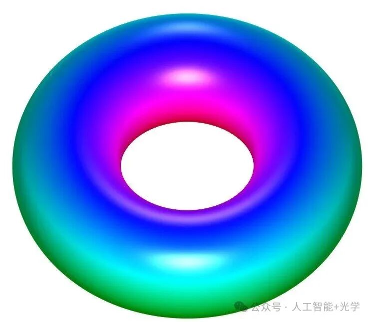

🌄 Python for Scalar Topological Vortex Plotting

import numpy as npimport matplotlib.pyplot as pltfrom mpl_toolkits.mplot3d import Axes3D# %% 1. Generate toroidal geometry dataR = 4  # Major radiusr = 1.8  # Minor radiusnum_pts = 200theta = np.linspace(0, 2 * np.pi, num_pts)phi = np.linspace(0, 2 * np.pi, num_pts)theta, phi = np.meshgrid(theta, phi)# Toroidal parametric equationsX = (R + r * np.cos(phi)) * np.cos(theta)Y = (R + r * np.cos(phi)) * np.sin(theta)Z = r * np.sin(phi)# %% 2. Define color mappingphase_shift = 2.5norm = plt.Normalize(vmin=0, vmax=2 * np.pi)C = norm(phi + phase_shift)# %% 3. Initialize window and plot surfacefig = plt.figure(figsize=(10, 7.5), facecolor='w')ax = fig.add_subplot(111, projection='3d')# Use colormap to get base colors (including Alpha channel)base_colors = plt.cm.hsv(C)# %% 4. Visual enhancement # 4.1 Hide axes and gridax.set_axis_off()ax.grid(False)# 4.2 Simulate lighting and material# Define light source positionslight_pos1 = np.array([0, -10, 10])light_pos2 = np.array([0, 10, 5])light_color2 = np.array([0.5, 0.5, 0.5])# Calculate surface normalsdx_dtheta = np.gradient(X, axis=1)dy_dtheta = np.gradient(Y, axis=1)dz_dtheta = np.gradient(Z, axis=1)dx_dphi = np.gradient(X, axis=0)dy_dphi = np.gradient(Y, axis=0)dz_dphi = np.gradient(Z, axis=0)nx = dy_dtheta * dz_dphi - dz_dtheta * dy_dphiny = dz_dtheta * dx_dphi - dx_dtheta * dz_dphinz = dx_dtheta * dy_dphi - dy_dtheta * dx_dphi# Normalize normalsnorm_n = np.sqrt(nx**2 + ny**2 + nz**2)norm_n[norm_n == 0] = 1 nx /= norm_nny /= norm_nnz /= norm_n# Simulate Phong lighting model# Ambient lightambient_strength = 0.5ambient_color = np.array([1.0, 1.0, 1.0])ambient = ambient_strength * ambient_color# Diffuse lightdiffuse_strength = 0.6l1 = light_pos1 / np.linalg.norm(light_pos1)dot_product1 = np.maximum(0, nx*l1[0] + ny*l1[1] + nz*l1[2])diffuse1 = diffuse_strength * dot_product1[..., np.newaxis]l2 = light_pos2 / np.linalg.norm(light_pos2)dot_product2 = np.maximum(0, nx*l2[0] + ny*l2[1] + nz*l2[2])diffuse2 = diffuse_strength * dot_product2[..., np.newaxis] * light_color2# Specular reflectionspecular_strength = 0.8specular_exponent = 15# View directionview_dir = np.array([1, 0, 1])# Calculate specular reflection for main light sourcereflect_dir1 = 2 * dot_product1[..., np.newaxis] * np.array([nx, ny, nz]).T - l1# Calculate dot product between view direction and reflectionspecular_dot = np.sum(reflect_dir1 * view_dir, axis=2)specular1 = specular_strength * np.maximum(0, specular_dot)**specular_exponent#  Combine final RGB colorfinal_color_rgb = ambient + (diffuse1 + diffuse2) + specular1[..., np.newaxis]final_color_rgb = np.clip(final_color_rgb, 0, 1)final_color_rgba = np.dstack((final_color_rgb, np.ones(final_color_rgb.shape[:2])))# Mix lighting effects with base colorslit_rgb = base_colors * final_color_rgbalit_rgb = np.clip(lit_rgb, 0, 1) # Ensure color values are valid# Plot surface and apply calculated colorsurf = ax.plot_surface(X, Y, Z, rstride=1, cstride=1, facecolors=lit_rgb,                       linewidth=0, antialiased=True, shade=False)# %% 5. Adjust view and add titleax.view_init(elev=45, azim=45)ax.set_title('Scalar Toroidal Vortex', fontsize=16, family='sans-serif')# Adjust axis proportions to be equalmax_range = np.array([X.max()-X.min(), Y.max()-Y.min(), Z.max()-Z.min()]).max() / 2.0mid_x = (X.max()+X.min()) * 0.5mid_y = (Y.max()+Y.min()) * 0.5mid_z = (Z.max()+Z.min()) * 0.5ax.set_xlim(mid_x - max_range, mid_x + max_range)ax.set_ylim(mid_y - max_range, mid_y + max_range)ax.set_zlim(mid_z - max_range, mid_z + max_range)# Show figureplt.show()# Recently used Linux system for plotting, readers can modify the save pathplt.savefig('/root/result.png') print("Image saved to /root/result.png")

✨ Follow us: Follow our public account “Artificial Intelligence + Optics” to learn practical skills

✨ Next article preview: “Creating Aesthetically Pleasing Vector Topological Vortex Surface Plots with Python & MATLAB”