Click the blue text above to follow us

📋📋📋 The table of contents is as follows: 🎁🎁🎁
Table of Contents
⛳️ Gift to Readers
💥1 Overview
1.1 Introduction
1.2 Application Scenarios
1.3 Method Implementation
📚2 Results
🎉3 References
🌈4 MATLAB Code, Data, Documentation

Gift to Readers
👨💻 Conducting research involves a profound system of thought, requiring researchers to be logical, meticulous, and serious. However, effort alone is not enough; often leveraging resources is more important than sheer hard work. Additionally, one must have innovative and inspirational points of view. When a philosophy teacher asks you what science is or what electricity is, do not dismiss these questions as trivial. Philosophy is the mother of science; it seeks to address ultimate questions and find those self-evident questions that only children would ask but you cannot answer. It is recommended that readers browse through the table of contents in order to avoid suddenly falling into a dark maze without finding their way back. This article may not reveal all the answers to your questions, but if it can spark clouds of doubt in your mind, it may create a beautiful sunset of thoughts. If it brings you a spiritual downpour, then take the opportunity to brush off the dust that has settled on your “lying flat” mindset. Perhaps, after the rain, the world will be clearer…🔎🔎🔎


1 Overview
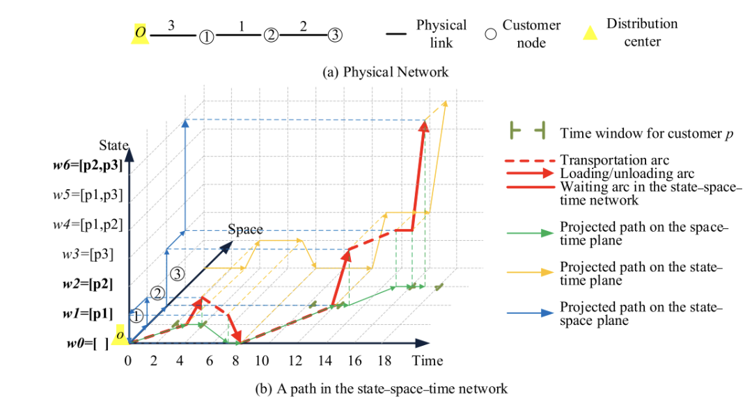
Abstract: Emerging urban logistics applications face numerous challenges, including complex traffic conditions and time-sensitive demands. This study considers a Vehicle Routing Problem with Time Windows (VRPTW) in the context of urban logistics, aiming to minimize total generalized costs, including transportation, waiting time, and fixed costs associated with each vehicle. We employ a high-dimensional spatiotemporal network flow model to construct a foundational vehicle routing problem (VRP) with rich criteria and constraints. A significant challenge in solving the VRP is how to iteratively improve the quality of primal and dual solutions and how to break the symmetry caused by many identical solutions, especially for homogeneous vehicles. Along this line, many coupling constraints, such as consensus constraints across different agents or decision-makers, need to be carefully handled to find high-quality optimal or near-optimal solutions for medium or large-scale instances. Currently, the Alternating Direction Method of Multipliers (ADMM) is widely used in the field of convex optimization as an integration of augmented Lagrangian relaxation and block coordinate descent methods for machine learning and large-scale continuous system optimization and control. In this work, we introduce the use of ADMM to solve the multi-vehicle routing problem, a special case of integer linear programming, and demonstrate a method to simplify the quadratic penalty term used in ADMM to a simple linear function. In a broader context, we develop a computationally reliable decomposition framework to iteratively improve the quality of primal and dual solutions. Essentially, the minimum cost path subproblem or other similar subproblems involving binary decisions can be embedded into a sequential solution scheme, outputting lower bound estimates and upper bound feasible solutions. We use classic Solomon VRP benchmark instances to test the performance of the proposed method. Our approach is also evaluated based on a real instance from a problem-solving competition of a major e-commerce company.
Keywords:Urban Logistics, Vehicle Routing Problem with Time Windows, Alternating Direction Method of Multipliers, Problem Decomposition

1.1 Introduction
-
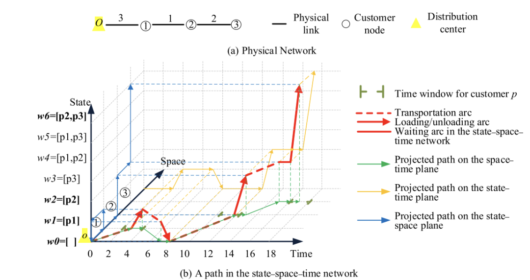
Augmented Lagrangian Relaxation (ALR): An augmented Lagrangian relaxation adds a quadratic penalty term to the Lagrangian relaxation, enhancing the robustness of the solution method and making the transformed problem easier to solve. Block Coordinate Descent Method: This algorithm performs a one-dimensional search along a coordinate direction during iterations to find a local minimum of the function, cycling through different coordinate directions. Alternating Direction Method of Multipliers (ADMM): ADMM can be used to iteratively optimize the VRPTW problem for K vehicles, allowing convergence from infeasible solutions to feasible ones. It decomposes the original problem into subproblems for each vehicle, enabling the use of forward dynamic programming algorithms to solve them.

1.2 Application Scenarios
-
Applicable to the Vehicle Routing Problem with Time Windows (VRPTW).

1.3 Method Implementation
FDP: Maintain a matrix (K, S, T), where K is the number of schemes considered, S is the number of demand points, and T is time. The state is the current time t, and the top K optimal delivery schemes. The state transition considers the top K optimal delivery schemes at the current time t, where for each scheme, any unserved customer can be selected. Upon reaching time t+t(i), where t(i) is the time cost from the current service point to the new customer i’s service point, the process jumps to time t+1. At each time t, only the top K optimal delivery schemes are considered. Define the initial state where all vehicles start from the same starting point at time 0. ADMM: First, initialize the upper and lower bounds of the original problem, Lagrange multipliers, quadratic term parameters, and the delivery schemes corresponding to each vehicle, then begin the loop. Fix the delivery paths of other vehicles and sequentially call FDP for K vehicles to find their minimum cost delivery paths, updating multipliers and penalty parameters, and then generate and update the bounds. CalculateCostForVehicle: In a given iteration, calculate the original cost for each vehicle based on the current fleet’s delivery scheme. FeasibleSolution: This is used to make the solution feasible after the iteration ends if the solution has not yet converged to a feasible solution. If a service point is served twice by two vehicles, retain the service of the second vehicle and modify the first vehicle’s delivery. If there are customers who have not been served, assign a spare vehicle to serve that customer. GeneralizedCostMatrix: Generate a generalized cost matrix that includes penalties for lateness added to the original cost matrix, allowing for lateness but incurring penalty costs. GenerateFreshness: Select the optimal fruit freshness for each vehicle so that the fruit is closest to the quality required by the customer upon delivery. Given the delivery schemes of each vehicle, loop through to try each freshness level to minimize the freshness deviation for each vehicle’s service customer, selecting the corresponding freshness.
📚2 Results The expected earliest delivery time window: 0 (default all vehicles start from time 0 from a common starting point) The expected latest delivery time window: Randomly generate delivery durations between two points in the time set: Randomly set the duration between any two points to 1, 2, or 3. Delivery cost ratio to duration: 1:1. Consumer order demand: Randomly set positive integers within the set [25, 40].

2 Results
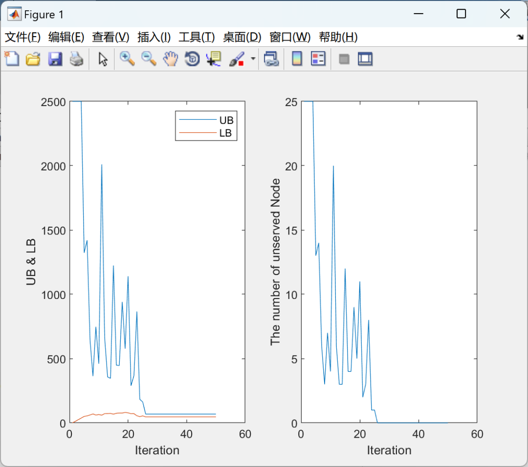
Figure 1: The left graph shows the changes in UB and LB with the number of iterations, while the right graph shows the number of unserved customers with the number of iterations. From the right graph, it can be seen that as the number of iterations increases, the number of unserved customers gradually decreases from the maximum value, converging to 0 around the 32nd iteration, indicating that the program gradually transitions from an infeasible solution where all customers are unserved to a feasible solution that meets all customer demands as the number of iterations increases. The left graph shows that as the number of iterations increases, the upper bound gradually decreases while the lower bound gradually increases, indicating that the quality of the solution improves with the number of iterations. Based on the above conclusions, as the number of iterations increases until the program converges, a good feasible solution can be obtained (or an approximate optimal solution can be obtained if it does not converge). Below, we compare the solutions from two iterations (one after convergence and one before convergence) to demonstrate that the solution after convergence is superior, indicating that the program can iteratively improve the solution until convergence.
We select the relatively well-computed result from the 14th iteration for analysis. The vehicle-path results and costs for the 14th iteration are shown in the table below (0 is the common starting point, 26 is the common endpoint):
|
Vehicle id |
Vehicle routing solution |
Cost |
|
1 |
0-26 |
0 |
|
2 |
0-26 |
0 |
|
3 |
0-23-18-26 |
5.0000 |
|
4 |
0-20-19-25-26 |
7.0000 |
|
5 |
0-5-2-12-26 |
5.0000 |
|
6 |
0-6-15-4-26 |
5.0000 |
|
7 |
0-20-8-25-26 |
6.0000 |
|
8 |
0-1-17-26 |
4.0000 |
|
9 |
0-11-16-7-26 |
5.0000 |
|
10 |
0-21-3-26 |
4.0000 |
|
11 |
0-24-9-10-26 |
6.0000 |
|
Total |
47.0000 |
Table 1: Vehicle Path Results and Costs for the 14th Iteration
Number of vehicles used: 9
Among them, customers served multiple times: 20.25
Unserved customers: 13.14.22
Detailed explanation can be found in Section 4.
%parameters
lambda1 = 1;
lambda2 = 1;
T = 10; % Time.
R = 4; % Freshness.
W = 100; % Car capacity.
c = 100; % Customers.
s = c+2; % Space node.
alpha2 = 2; % Time window penalty for delivery late.
rho = 0.1;
bestK = 100;
iteration = 100; % ADMM iterations.
% The next 3 lines of code are used to generate random time intervals
% between random 2 nodes. Writes it in an excel file and then copy it
% to 'inputFor100.xlsx' file.
%timeRange = [1, 3];
%[ B ]  =  GenerateRandomTime( c, timeRange );
%xlswrite('randomTimeFor100', B);
node = xlsread('inputFor100.xlsx', 1, 'B2:E101', 'basic');
demand = node(:, 1);
%et = node(:, 2);
lt = node(:, 3);
freshness = node(:, 4);
K = ceil(sum(demand)/W)+2; % Set vehicle number.
clear node;
link = xlsread('inputFor100.xlsx', 2, 'D2:D10405', 'basic');
link = reshape(link, [s, s]);
[ UB1 ] = CalculateObject1UB( link );
link = reshape(link, [s, s, 1, 1]);
C = zeros(s, s, T+1, T+1); % Arc cost matrix. Vehicles start from t=0......
subplot(1, 2, 1)
plot(x, y1, x, y2);
xlabel('Iteration')
ylabel('UB & LB')
legend('UB','LB')
subplot(1, 2, 2)
plot(x, unServedNode);
xlabel('Iteration')
ylabel('The number of unserved Node')
% Suggest to use this function after program has been converged.
[ finalSeq, timeSeq ] = FeasibleSolution( visitedSeq, finalRout, serviceTimes, C );
% Generate freshness deviation and freshness choice for each vehicle.
[ proposalR_K, freshnessDeviation ] = ...
    GenerateFreshness( finalSeq, timeSeq, freshness, R );

3References
Some content in this article is sourced from the internet, and references will be noted. If there are any inaccuracies, please feel free to contact us for removal.

[1] Y. Yao, X. Zhu, H. Dong, S. Wu, H. Wu, L. C. Tong, and X. Zhou, “ADMM-based Problem Decomposition Scheme for Vehicle Routing Problem with Time Windows,” Transportation Research Part B: Methodological, vol. 129, no. 19, pp. 156-174, 2019.

4 MATLAB Code, Data, Documentation
Public Account Lychee Research Society