💥💥💞💞Welcome to this blog❤️❤️💥💥
🏆Author’s Advantage: 🌞🌞🌞The blog content aims to be logically coherent and clear for the convenience of readers.
⛳️Motto: A journey of a hundred miles begins with a single step.
⛳️Gift to Readers
👨💻Conducting research involves a profound system of thought, requiring researchers to be logical and diligent, but effort alone is not enough; leveraging resources is often more important. Additionally, one should have innovative ideas and inspirations. Readers are advised to browse in order to avoid suddenly falling into a dark maze without finding their way back. This content may not reveal all the answers to your questions, but if it can clarify the doubts rising in your mind, it may create a beautiful sunset of insights. If it brings you a storm in your spiritual world, then take the opportunity to brush off the dust that has settled on your ‘lying flat’ mindset.
Perhaps, after the rain, the sky will be clearer…….🔎🔎🔎
💥1 Overview
Research on crack detection and marking in images
1. Basic Principles and Technical Methods of Crack Detection
Crack detection technology can be divided into two main categories based on principles: traditional physical detection and intelligent detection based on image processing/deep learning.
1.1 Traditional Physical Detection Methods
Visual Inspection
Principle: Direct observation of surface cracks with the naked eye or magnifying devices, suitable for visible macro cracks.
Advantages: Simple operation, low cost.
Disadvantages: Relies on subjective judgment, unable to detect small or internal cracks.
Magnetic Particle Inspection (MPI)
Principle: Uses a magnetic field to attract magnetic powder to surface cracks in ferromagnetic materials, forming visible traces.
Applicability: Only suitable for ferromagnetic materials, high sensitivity (surface and near-surface cracks).
Limitations: Ineffective for non-magnetic materials, complex operation.
Dye Penetrant Testing
Principle: Penetrant liquid seeps into cracks, and developer reveals open cracks.
Applicability: Complex workpieces with smooth surfaces.
Disadvantages: Poor effectiveness on coated surfaces, penetrant liquid may be toxic.
Ultrasonic Testing
Principle: High-frequency sound waves reflect within the material, analyzing echoes to determine crack location and depth.
Advantages: Can detect internal and deeply buried cracks, suitable for metals, composites, etc.
Challenges: Requires specialized equipment and operators, surface must be smooth.
Laser Speckle Detection
Principle: Uses changes in speckle patterns formed by laser interference to detect surface micro-deformations.
Advantages: Non-contact, high sensitivity (nanometer-level cracks).
Disadvantages: High equipment cost, complex operation.
2. Image Processing-Based Crack Detection Algorithms
2.1 Traditional Image Processing Techniques
Preprocessing Techniques
Filtering and Denoising: Median filtering, wavelet transform.
Image Enhancement: Ridge wavelet enhancement, contrast stretching.
Edge Detection and Segmentation
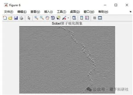
Operator Methods: Sobel, Canny, Roberts operators.

Threshold Segmentation: Otsu’s algorithm, adaptive threshold.
Morphological Processing: Dilation, erosion to connect broken cracks.
Parameter Calculation
Skeletonization: Eight-neighborhood thinning algorithm to extract single-pixel skeletons.
Length/Width Calculation: Based on pixel statistics or curve fitting.
Limitations: Easily affected by lighting and noise, poor robustness against complex backgrounds (e.g., water stains, scratches).
2.2 Deep Learning-Based Algorithms
Mainstream Model Architectures
Classification Models: ResNet, EfficientNet for determining the presence of cracks.
Object Detection: YOLO series, Faster R-CNN for locating crack areas.
Semantic Segmentation: U-Net, DeepLab for pixel-level extraction.
Innovative Technologies
Transfer Learning: Fine-tuning pre-trained models (e.g., ResNet50) to reduce data requirements.
Attention Mechanism: Spatial attention enhances feature focusing capability.
Multi-Scale Fusion: Combining features from different levels to enhance detection robustness.
Lightweight Design: EfficientNet optimizes computational efficiency for mobile adaptation.
Performance Comparison
Accuracy: Improved U-Net’s mPA reaches 90.08%, Attention-ResNet50-GA model F1 score 0.9983.
Speed: YOLOv5 achieves real-time detection on drone platforms.
3. Detection Accuracy Evaluation Metrics and Standards
3.1 Physical Detection Accuracy Standards
Crack Width: Reading accuracy ±0.001 mm.
Crack Depth: Error ≤ ±5% (error ±5 mm when depth < 50 mm).
Sound Time Measurement: Relative error ≤ ±1.0%.
3.2 Algorithm Performance Metrics
Classification/Detection Metrics


Segmentation Metrics
IoU (Intersection over Union): 

mIoU: Mean IoU for multiple categories.
Kappa Coefficient: Measures annotation consistency.
Actual Cases
DeepCrack: F-measure reaches 0.87.
1D-CNN-LSTM: Test set accuracy 99.25%.
4. Challenges and Future Directions
Current Challenges
Data Bottleneck: Difficulty in obtaining pixel-level annotated datasets.
Complex Environments: Lighting changes and background noise affect algorithm robustness.
Real-Time Performance: Insufficient processing speed for high-resolution images.
Future Trends
Multi-Modal Fusion: Combining data from infrared, ultrasonic, and other sensors to enhance detection dimensions.
Self-Supervised Learning: Reducing dependence on annotated data.
Edge Computing: Deploying lightweight models on drones and mobile devices.
Explainability: Breaking through the “black box” limitation to enhance model transparency.
5. Conclusion
Crack detection technology is evolving from traditional physical methods to intelligent and automated approaches. Deep learning (especially models like U-Net and YOLO) has significantly improved detection accuracy in complex environments, while open-source tools and industrial-grade systems (such as drones + deep learning) are driving practical applications. Future breakthroughs are needed in data generation, model lightweighting, and multi-modal fusion to achieve more efficient and cost-effective crack health monitoring.
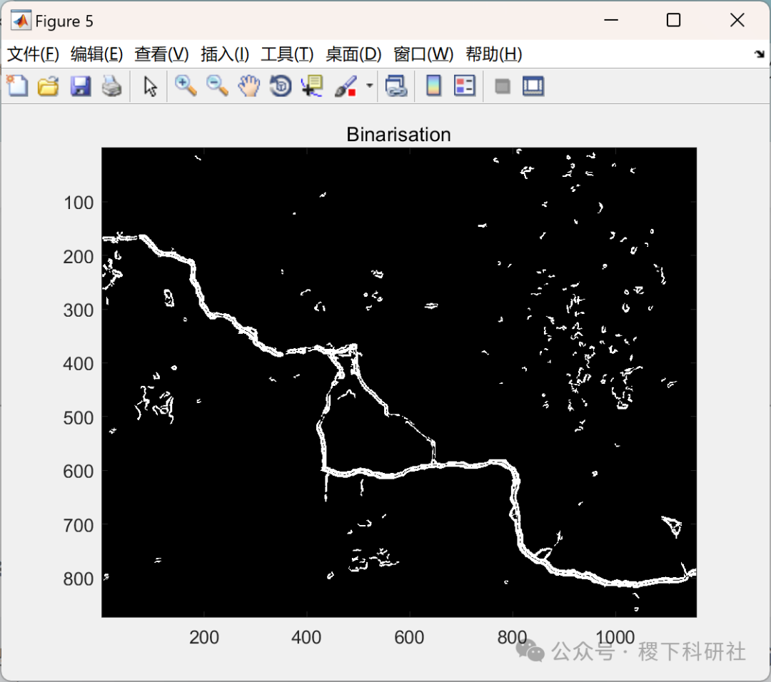
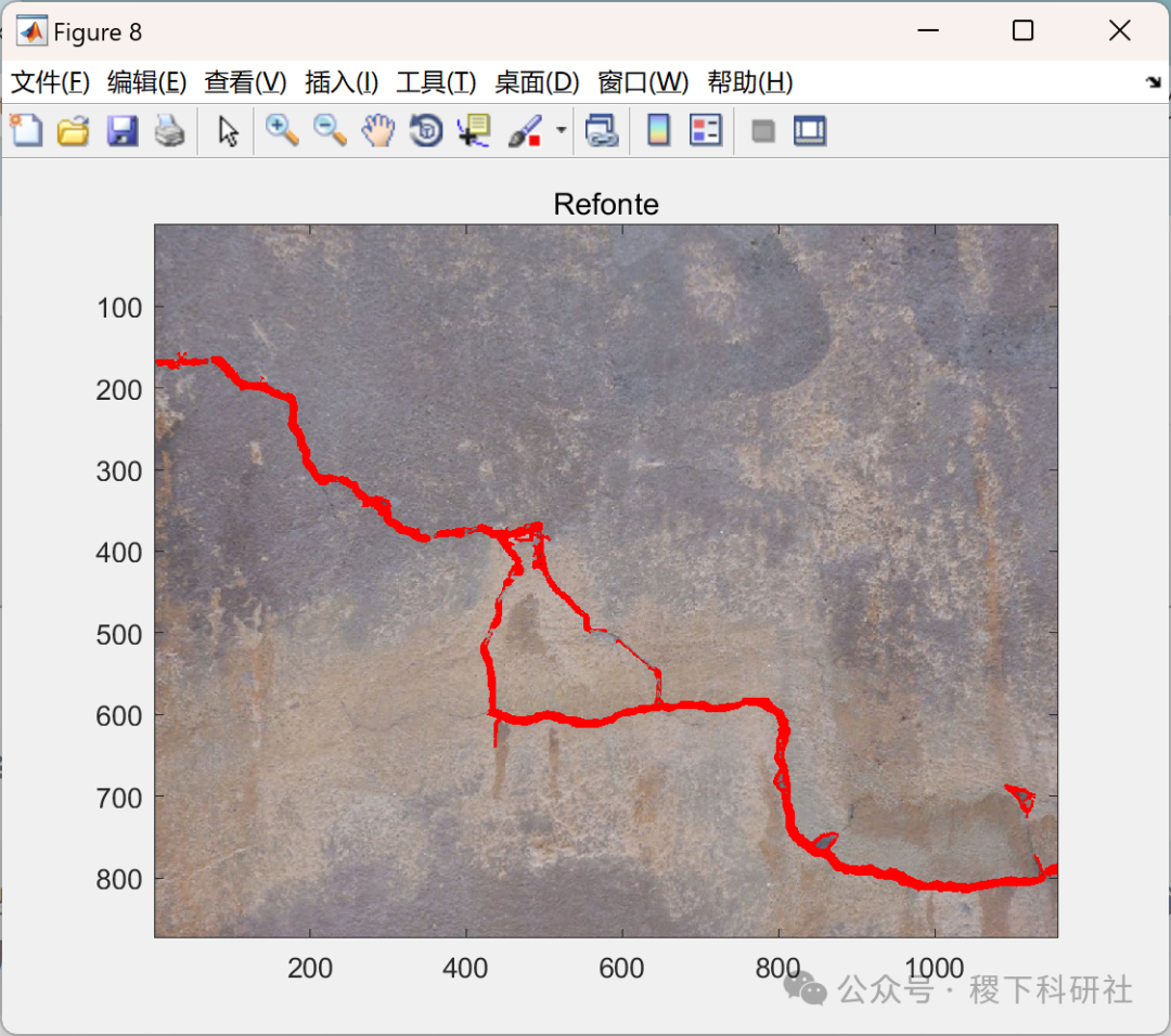
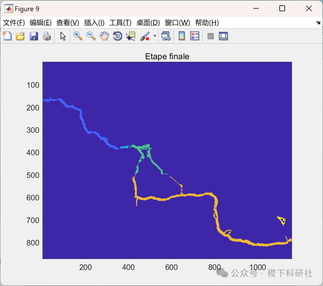
📚2 Running Results


Main function code:
clear allclose all% clfI=imread(‘exemple2.PNG’);Indg=rgb2gray(I); %NdG[l,c]=size(Indg); %Size of Indg matrix%—-Smoothing————G = fspecial(‘gaussian’,[5 5],3); %create Gaussian filterIG = imfilter(Indg,G,’symmetric’,’same’,’conv’); %Gaussian filtering%————————–%————Gradient Calculation—–%Gradient matricesIX=zeros(l,c);%horizontal gradIY=zeros(l,c);%vertical gradIXY=zeros(l,c);%norm grad%Sobel 3x3for i=2:l-1 for j=2:c-1 IX(i,j)=-(-double(IG(i-1,j-1))-2double(IG(i,j-1))-double(IG(i+1,j-1))+double(IG(i-1,j+1))+2double(IG(i,j+1))+double(IG(i+1,j+1)))/8; IY(i,j)=-(-2double(IG(i-1,j))+2double(IG(i+1,j))-double(IG(i-1,j-1))+double(IG(i+1,j-1))-double(IG(i-1,j+1))+double(IG(i+1,j+1)))/8; IXY(i,j)=sqrt(((IX(i,j))^2)+((IY(i,j))^2)); endend%——-Binarization—-%Hysteresis thresholdingIbin=zeros(l,c);%binarySh=8;Sb=5;for i=1:l for j=1:c if IXY(i,j)>=Sh %Threshold: gradient > Sh Ibin(i,j)=255; elseif IXY(i,j)<sb %threshold: gradient < sb = ibin(i,j)=”0;” end=” endendfor=” p=”1:50″ for=” i=”1:l” j=”1:c” if=” ixy(i,j)=Sb %Threshold: Sh > gradient > Sb % Extraction of 8 neighboring pixels vect = [Ibin(i-1,j-1:j+1) Ibin(i, j-1) Ibin(i, j+1) Ibin(i+1,j-1:j+1)]; if max(vect)==255 Ibin(i,j)=255; else Ibin(i,j)=0; end end end endend %———-Identification of regions—–[L,num]=bwlabel(Ibin,8);t=regionprops(L, ‘area’); %info on the regionssize=zeros(num,1);for g=1:num size(g,1)=t(g,1).Area(1,1); %Extract the size of the regionsend%—–Removal of small regions——Ifer=zeros(l,c);for i=1:l for j=1:c for k=1

clear all
close all
% clf
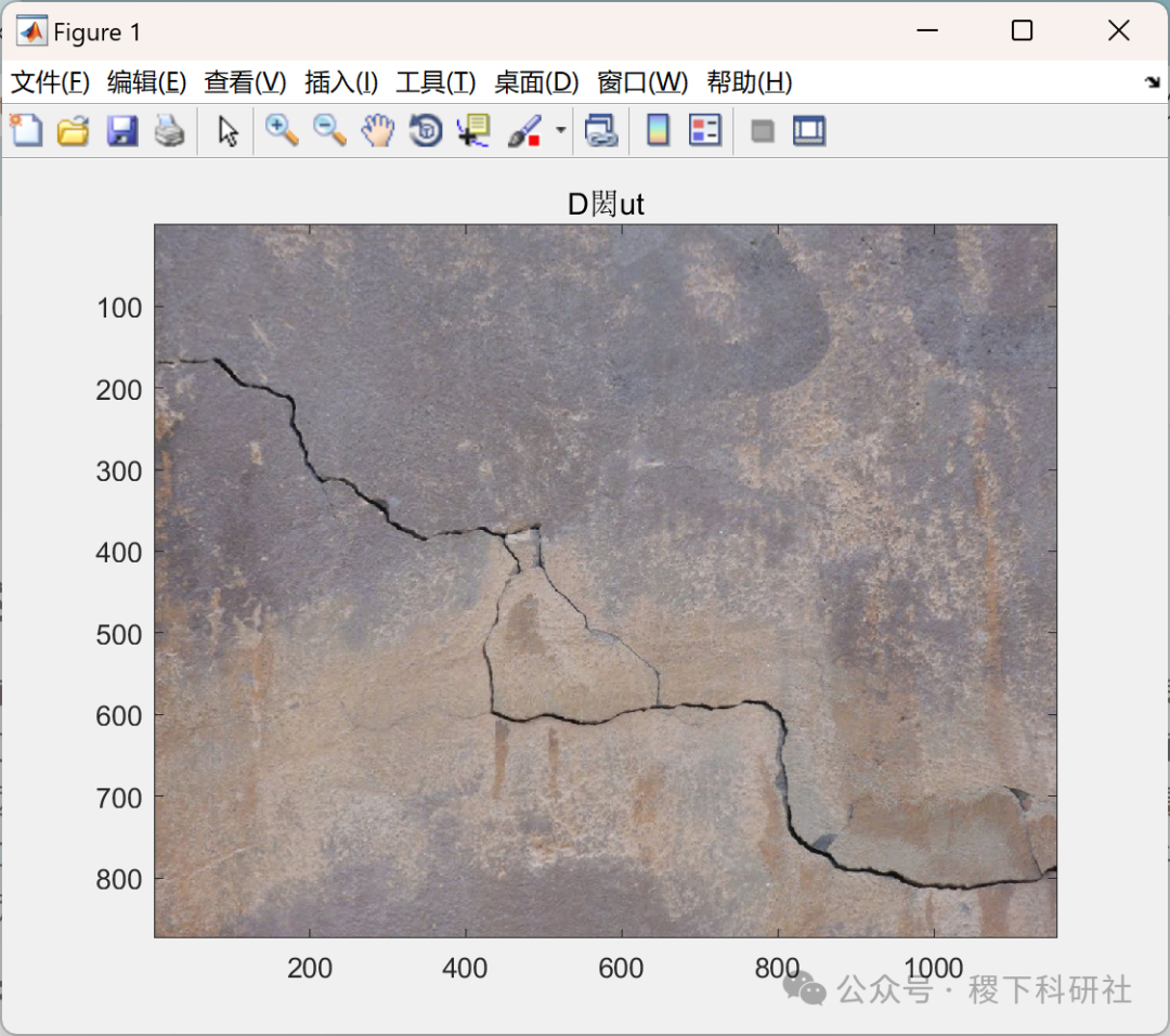
I=imread(‘exemple2.PNG’);
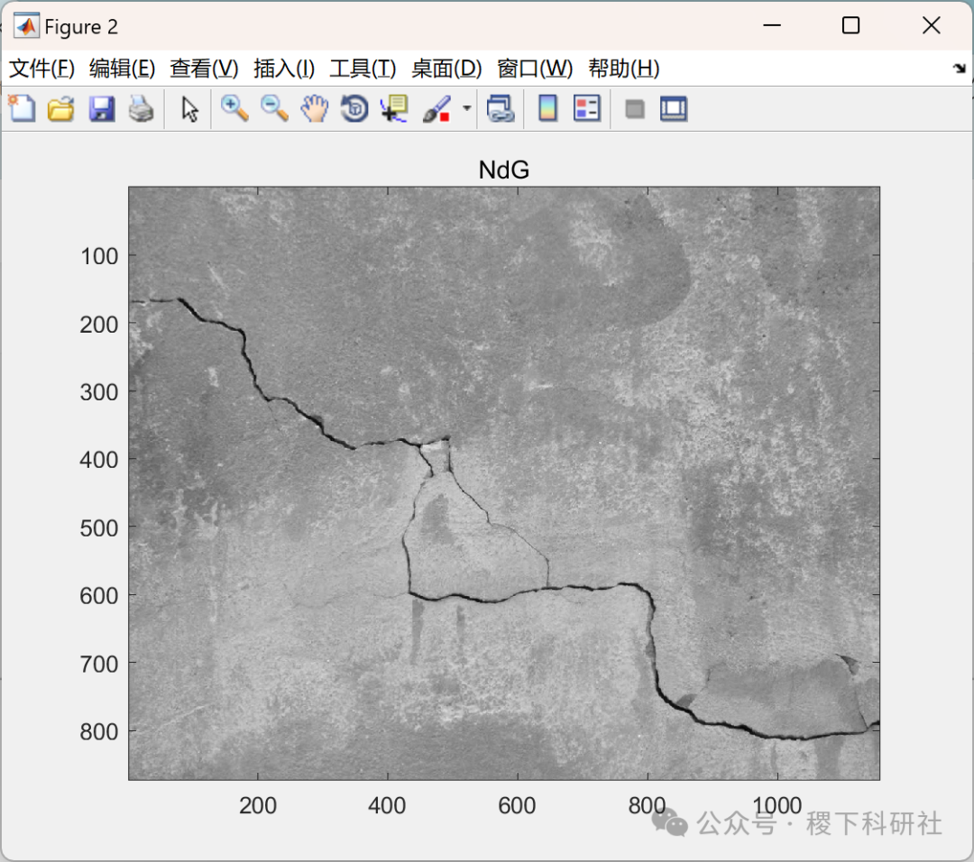
Indg=rgb2gray(I); %NdG
[l,c]=size(Indg); %Size of Indg matrix
%—-Smoothing————
G = fspecial(‘gaussian’,[5 5],3); %create Gaussian filter
IG = imfilter(Indg,G,’symmetric’,’same’,’conv’); %Gaussian filtering
%————————–
%————Gradient Calculation—–
%Gradient matrices
IX=zeros(l,c);%horizontal grad
IY=zeros(l,c);%vertical grad
IXY=zeros(l,c);%norm grad
%Sobel 3×3
for i=2:l-1
for j=2:c-1
IX(i,j)=-(-double(IG(i-1,j-1))-2double(IG(i,j-1))-double(IG(i+1,j-1))+double(IG(i-1,j+1))+2double(IG(i,j+1))+double(IG(i+1,j+1)))/8;
IY(i,j)=-(-2double(IG(i-1,j))+2double(IG(i+1,j))-double(IG(i-1,j-1))+double(IG(i+1,j-1))-double(IG(i-1,j+1))+double(IG(i+1,j+1)))/8;
IXY(i,j)=sqrt(((IX(i,j))^2)+((IY(i,j))^2));
end
end
%——-Binarization—-
%Hysteresis thresholding
Ibin=zeros(l,c);%binary
Sh=8;
Sb=5;
for i=1:l
for j=1:c
if IXY(i,j)>=Sh %Threshold: gradient > Sh
Ibin(i,j)=255;
elseif IXY(i,j)<Sb %Threshold: gradient < Sb
Ibin(i,j)=0;
end
end
end
for p=1:50
for i=1:l
for j=1:c
if IXY(i,j)<Sh && IXY(i,j)>=Sb %Threshold: Sh > gradient > Sb
% Extraction of 8 neighboring pixels
vect = [Ibin(i-1,j-1:j+1) Ibin(i, j-1) Ibin(i, j+1) Ibin(i+1,j-1:j+1)];
if max(vect)==255
Ibin(i,j)=255;
else
Ibin(i,j)=0;
end
end
end
end
end
%———-Identification of regions—–
[L,num]=bwlabel(Ibin,8);
t=regionprops(L, ‘area’); %info on the regions
size=zeros(num,1);
for g=1:num
size(g,1)=t(g,1).Area(1,1); %Extract the size of the regions
end
%—–Removal of small regions——
Ifer=zeros(l,c);
for i=1:l
for j=1:c
for k=1
🎉3 References
Some content in this article is sourced from the internet, and references will be noted. If there are any inaccuracies, please feel free to contact for removal. (The content is for reference only, and specific results are subject to running outcomes)
[1] Guo Yi, Wu Qiong. Efficient Detection Algorithm for Micro-Cracks on Ship Hull Surfaces under Visual Image Processing [J]. Ship Science and Technology, 2021, 43(18): 1-3.
🌈4 Matlab Code Implementation
Data acquisition, more fan benefits, MATLAB|Simulink|Python resource acquisition


Reply in the public account: Program download