Post-Processing of One-Dimensional Wave Spectrum Using MATLAB and SWAN Model

Reading SWAN Spectrum Files and Plotting Wave Spectra in MATLAB

In coastal and ocean numerical simulations, the SWAN model is frequently used for wave calculations. It outputs a standard spectrum file (<span>.spc</span>) that records information such as frequency and energy spectrum density. The following MATLAB code demonstrates how to read and plot the one-dimensional wave spectrum from SWAN.

First, we read the file information:

1️⃣ File Reading

filename = '1D_point.spc';   % SWAN output spectrum file
fid = fopen(filename,'r');

👉 Open the specified SWAN spectrum file and prepare to read.

2️⃣ Reading Frequency Information

while true
    tline = fgetl(fid);
    if contains(tline,'AFREQ')   % Find the AFREQ keyword
        break;
    end
end

line = fgetl(fid);
tokens = textscan(line,'%f');
nFreq = tokens{1}(1);     % Number of frequencies

👉 The SWAN file defines the number of frequencies and their specific values after AFREQ. The code reads line by line and stores all frequencies in the <span>freq</span> array.

3️⃣ Reading Spectrum Quantities (QUANT)

while true
    tline = fgetl(fid);
    if contains(tline,'QUANT')
        break;
    end
end

line = fgetl(fid);
nQuant = sscanf(line, '%f', 1);  % Number of spectrum quantities

👉 SWAN defines the output spectrum quantities (such as energy density, direction, etc.) in the QUANT section. Here, we mainly use the variance density from the first column (VaDens).

4️⃣ Reading Time and Measurement Point Data

date_line = strtrim(fgetl(fid));  % Time, e.g., 20240720.000000
nLoc = 5;   % Number of measurement points defined in the file
spectra = nan(nFreq,nLoc);

👉 Each measurement point has a set of spectrum data, which is read in a loop and saved as a <span>spectra</span> matrix.

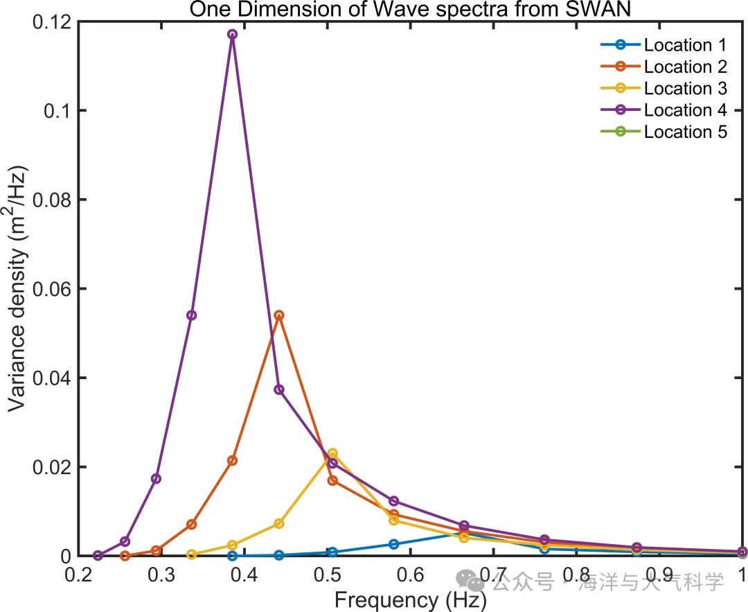
5️⃣ Plotting the Spectrum

figure('position',[5050850650],'color','w');
for loc = 1:nLoc
    plot(freq, spectra(:,loc),'-o',
    'DisplayName',['Location ',num2str(loc)],'linewidth',2);
end
xlabel('Frequency (Hz)');
ylabel('Variance density (m^2/Hz)');
title('One Dimension of Wave spectra from SWAN');
legend show;

👉 The x-axis represents frequency (Hz), and the y-axis represents variance density (m²/Hz).

.rtcContent { padding: 30px; }
.lineNode {font-size: 12pt; font-family: "Times New Roman", Menlo, Monaco, Consolas, "Courier New", monospace; font-style: normal; font-weight: normal; }
clear;clc;close all;%  Read SWAN standard spectrum file and plot wave spectrum
filename = '1D_point.spc';   % Your SWAN output file name
fid = fopen(filename,'r');
if fid<0    error('Cannot open file %s', filename);end
% ---- Jump to AFREQ ----
while true    tline = fgetl(fid);
    if contains(tline,'AFREQ')        break;    end
end
line = fgetl(fid);
tokens = textscan(line,'%f');   % Read only numeric values
nFreq = tokens{1}(1);           % The first number is the number of frequencies
freq = zeros(nFreq,1);
for i = 1:nFreq    freq(i) = str2double(fgetl(fid));end
% ---- Jump to QUANT ----
while true    tline = fgetl(fid);
    if contains(tline,'QUANT')        break;    end
end
clear line
line = fgetl(fid);
nQuant = sscanf(line, '%f', 1);  % Read only the first number
% Skip description lines
for i=1:(nQuant*3)    fgetl(fid);end
% ---- Read Time ----
date_line = strtrim(fgetl(fid));  % e.g., 20240720.000000
% ---- Read each measurement point's data ----
nLoc = 5;   % Defined by LONLAT in the file
spectra = nan(nFreq,nLoc);
for loc = 1:nLoc    tline = fgetl(fid);   % LOCATION n
    data = nan(nFreq,nQuant);    for i = 1:nFreq        vals = str2num(fgetl(fid)); %#ok<ST2NM>        if isempty(vals)            continue;        end        data(i,:) = vals;    end
    % Take the first column VaDens    spectra(:,loc) = data(:,1);end
fclose(fid);% close file
% miss value is nanspectra(spectra==-99)=nan;% ---- Plot ----
close all
figure('position',[50 50 850 650],'color','w');hold on; box on;
for loc = 1:nLoc    plot(freq, spectra(:,loc),'-o','DisplayName',['Location ',num2str(loc)],'linewidth',2);end
xlabel('Frequency (Hz)');
ylabel('Variance density (m^2/Hz)');
legend show;
legend Box off
title('One Dimension of Wave spectra from SWAN');
set(gca,'linewidth',2,'fontname','arial','fontsize',15)
export_fig('one_point.jpg','-r600')