🔍See the end of the article for program acquisition methods
📶The work includes complete programs, documentation, references, and operation videos
🌠Preview of Simulation Conclusions
Testing results using Matlab 2024b are as follows: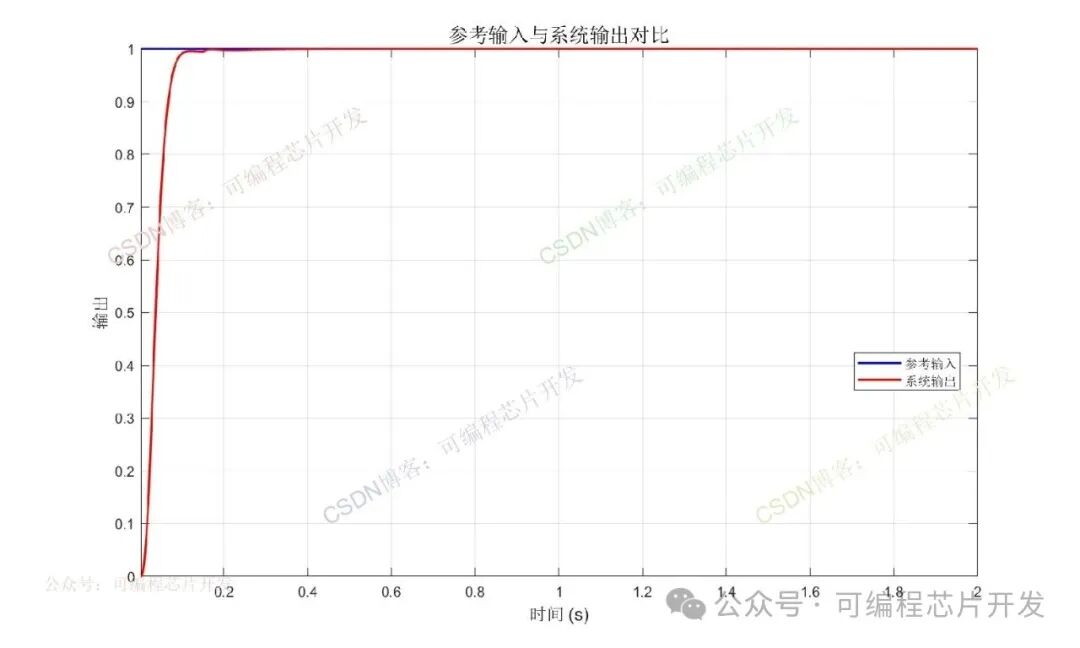
 ⚡Program Function Description
<span><span>The functions and principles of this program are as follows:</span></span>
CMAC is a lookup table-based local approximation network, whose structure mimics the cerebellum’s “parallel distributed processing” mechanism. Its core advantages are reflected in two aspects:
Local Generalization Ability: CMAC only activates a small number of neurons (storage units) related to the input, rather than activating the entire network. The learning process updates only local weights, significantly improving learning speed to meet real-time control requirements;
Strong Fault Tolerance: A failure of a single storage unit only affects the local input area and does not cause the entire control system to fail, making it suitable for harsh industrial environments;
No Need for Precise Mathematical Models: The system’s unknown dynamics can be approximated through sample learning without the need to establish a nonlinear mathematical model of the controlled object in advance, lowering the engineering application threshold.
✨Partial Program
<span><span>Some core program content is as follows</span></span>
figure;% Adjust timesteady_state = sim_data.rin(end);tolerance = 0.05 * steady_state;stable_idx = find(abs(sim_data.yout - steady_state) <= tolerance, 1, 'first');performance.settling_time = sim_data.time(stable_idx);%% 6. Display performance indicatorsfprintf('Control system performance indicators:
');fprintf('1. Steady-state error: %.6f
', performance.steady_state_error);fprintf('2. Mean Squared Error (MSE): %.6f
', performance.mse);fprintf('3. Integral Absolute Error (IAE): %.6f
', performance.iae);fprintf('4. Integral Time Absolute Error (ITAE): %.6f
', performance.itae);fprintf('5. Overshoot: %.2f%%
', performance.overshoot);fprintf('6. Rise time: %.4f seconds
', performance.rise_time);fprintf('7. Settling time: %.4f seconds
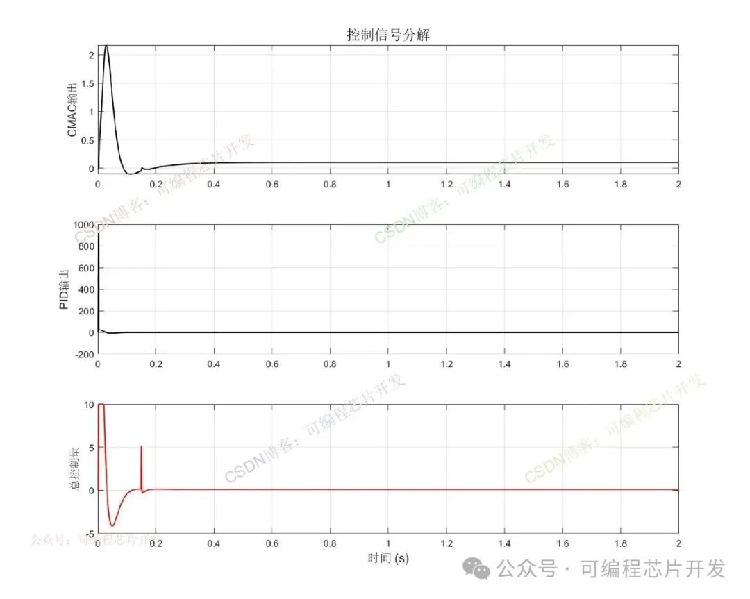
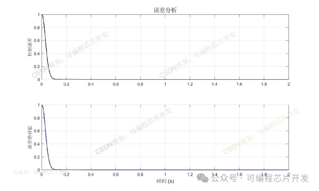
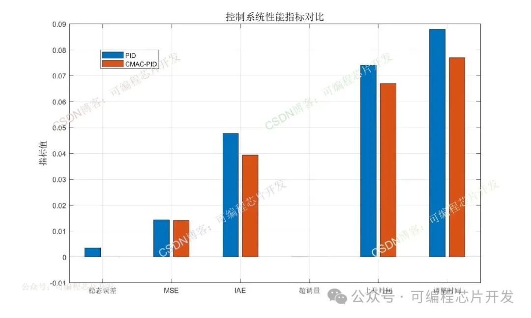
', performance.settling_time);%% 7. Result Visualization% Figure 1: Reference input and system outputfigure('Name', 'System Tracking Performance', 'Position', [100, 100, 1000, 600]);plot(sim_data.time, sim_data.rin, 'b-', 'LineWidth', 1.5);hold on; grid on;plot(sim_data.time, sim_data.yout, 'r-', 'LineWidth', 1.5);xlabel('Time (s)', 'FontSize', 12);ylabel('Output', 'FontSize', 12);title('Comparison of Reference Input and System Output', 'FontSize', 14);legend('Reference Input', 'System Output', 'Location', 'Best');axis tight;% Figure 2: Control signalfigure('Name', 'Control Signal', 'Position', [100, 200, 1000, 800]);subplot(3,1,1);plot(sim_data.time, sim_data.un, 'k-', 'LineWidth', 1.2);grid on;ylabel('CMAC Output', 'FontSize', 11);title('Control Signal Decomposition', 'FontSize', 14);subplot(3,1,2);plot(sim_data.time, sim_data.up, 'k-', 'LineWidth', 1.2);grid on;ylabel('PID Output', 'FontSize', 11);subplot(3,1,3);plot(sim_data.time, sim_data.u, 'r-', 'LineWidth', 1.2);grid on;xlabel('Time (s)', 'FontSize', 12);ylabel('Total Control Amount', 'FontSize', 11);% Figure 3: Error Analysisfigure('Name', 'Error Analysis', 'Position', [100, 300, 1000, 600]);subplot(2,1,1);plot(sim_data.time, sim_data.error, 'k-', 'LineWidth', 1.2);grid on;ylabel('Control Error', 'FontSize', 11);title('Error Analysis', 'FontSize', 14);subplot(2,1,2);plot(sim_data.time, abs(sim_data.error), 'b-', 'LineWidth', 1.2);grid on;xlabel('Time (s)', 'FontSize', 12);ylabel('Absolute Error', 'FontSize', 11);% Figure 4: Performance Indicator Bar Chartfigure('Name', 'Performance Indicators', 'Position', [100, 400, 1000, 600]);metrics1 = [performance.steady_state_error, performance.mse, ... performance.iae, performance.overshoot/100, ... performance.rise_time, performance.settling_time];load R0.matmetrics2 = metrics;bar([metrics2;metrics1]');grid on;ylabel('Indicator Value', 'FontSize', 12);title('Comparison of Control System Performance Indicators', 'FontSize', 14);set(gca, 'XTickLabel', {'Steady-state Error', 'MSE', 'IAE', 'Overshoot', 'Rise Time', 'Settling Time'});legend('PID','CMAC-PID');130🌍Program Acquisition Method
Click the bottom left corner of WeChat to read the original text