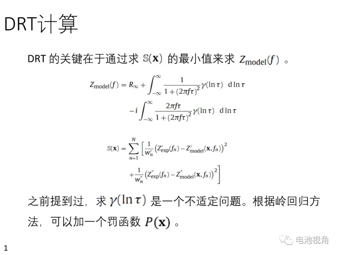
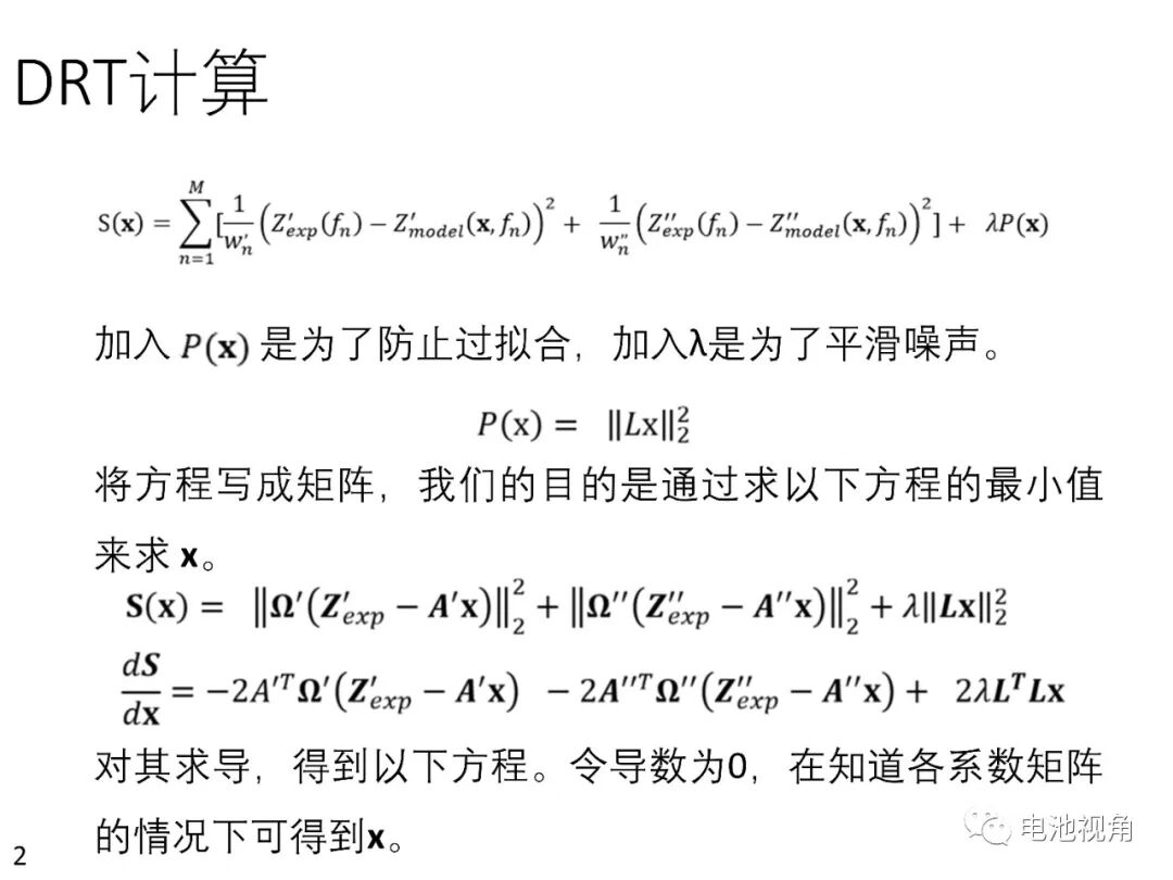
After understanding the basic concept of DRT, the remaining question is how to determine the time distribution function. It was previously mentioned that directly finding the minimum of S(x) to obtain the time distribution function is an ill-posed problem. To address this issue, we use ridge regression to handle the overfitting problem. This method introduces a penalty function λP(x), resulting in a new S(x), and then we find the minimum of the new S(x). The parameter λ can eliminate noise but may also introduce bias. Therefore, selecting λ must be done carefully.
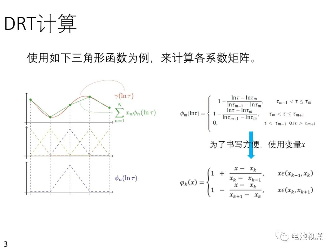
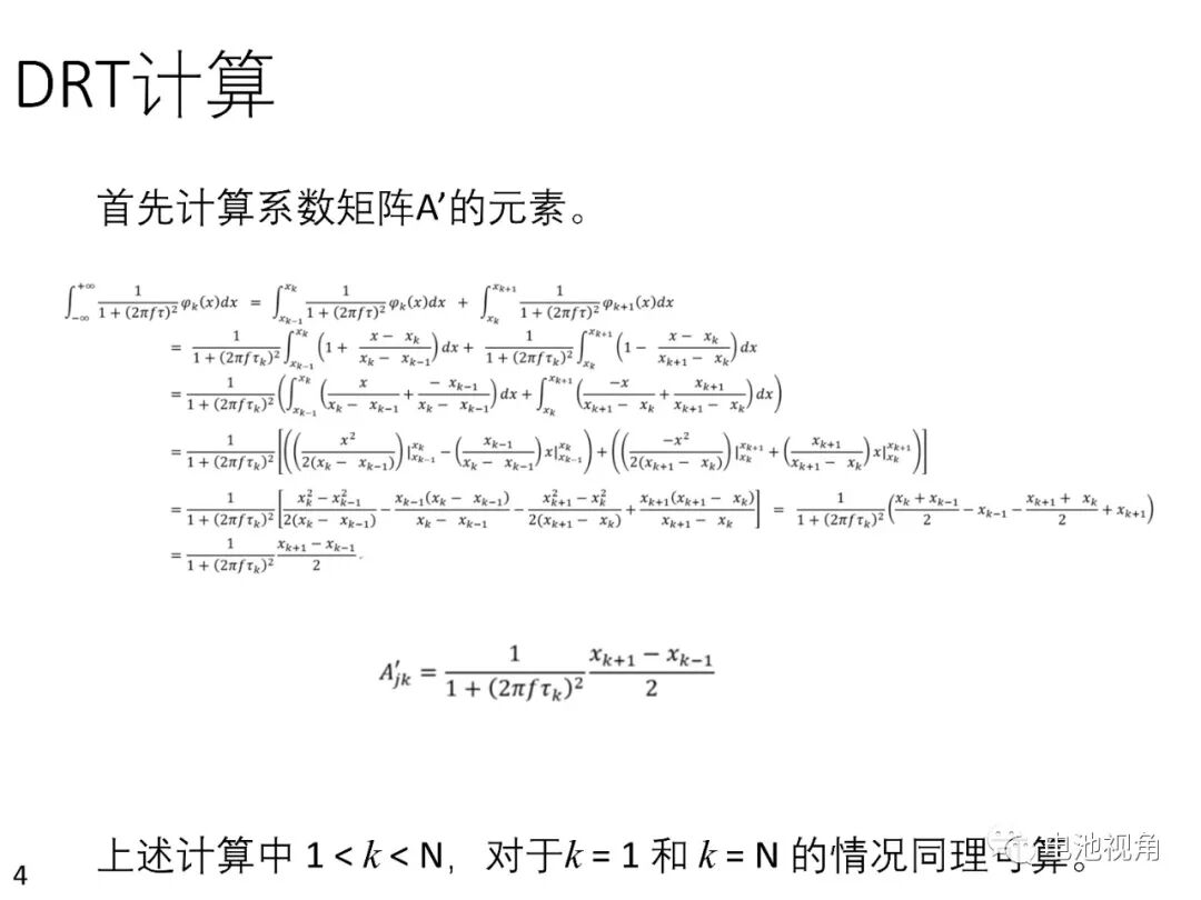
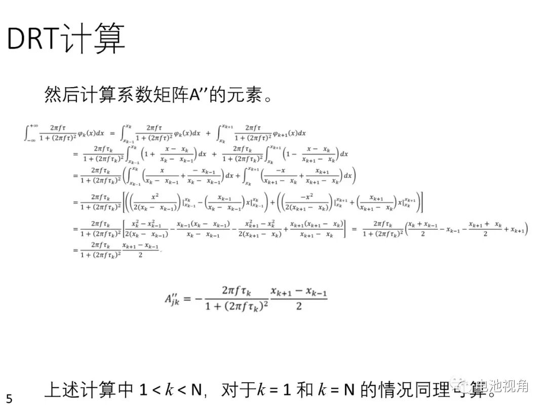
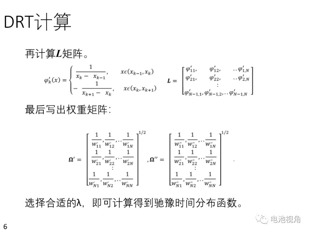
We first obtain the coefficients of the basis function x and the test results Zexp, the basis function φ, the penalty function P, and the weights ω, and λ by setting the derivative of the new S(x) equal to 0. Then, using the triangular basis function as an example, we calculate the corresponding matrix and subsequently compute the coefficients of the time distribution function, thus obtaining the time distribution function.
This section details the transformation from expressions to matrices, the calculation of matrix elements, the computation of the penalty function, etc. Through this introduction, we can easily implement DRT and use DRT to help us analyze the impedance spectrum.