Full text download link: http://tecdat.cn/?p=27340

Volatility is an important concept with many applications in finance and trading. It is the basis for option pricing. Volatility also allows you to determine asset allocation and calculate the Value at Risk (VaR) of a portfolio. (Click “Read the original” at the end for complete code data ) .

Even volatility itself is a financial instrument, such as the CBOE VIX volatility index. However, unlike security prices or interest rates, volatility cannot be directly observed. Instead, it is often measured as the statistical volatility of the historical returns of a security or market index. This type of measure is called realized volatility or historical volatility. Another way to measure volatility is through the options market, where option prices can be used to derive the volatility of the underlying security through certain option pricing models. The Black-Scholes model is the most popular model. This type of definition is called implied volatility. The VIX is based on implied volatility.

Related Videos

There are various statistical methods to measure the historical volatility of return series. High-frequency data can be used to calculate the volatility of low-frequency returns. For example, using intraday returns to calculate daily volatility; using daily returns to calculate weekly volatility. Daily OHLC (Open, High, Low, Close) can also be used to calculate daily volatility. Academic methods include ARCH (Autoregressive Conditional Heteroskedasticity), GARCH (Generalized ARCH), TGARCH (Threshold GARCH), EGARCH (Exponential GARCH), etc. We will not discuss each model and its pros and cons in detail. Instead, we will focus on the Stochastic Volatility (SV) model and compare its results with other models. Generally, SV models are difficult to estimate using regression methods, as we will see in this article.

EUR/USD Exchange Rate

We will take the daily quotes of the EUR/USD exchange rate from 2003 to 2018 as an example to calculate daily volatility.

subplot(2,1,1);plot(ta,csl)subplot(2,1,2);plot(at,rtdan);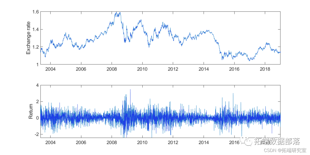

Figure 1. Top: Daily exchange rate (ask) of EUR/USD. Bottom: Daily log return percentage.

Figure 2 shows the basis for the absence of serial correlation in returns.

[sdd,slodgdL,infaso] = estimaadte(Mddsdl,rtasd);[aEass,Vad,lsagLd] = infer(EstMsssddl,rtsdn);[hsd,pValasdue,dstat,ascValue] = lbqtest(reas,'lags',12)[hs,pdValsue,sdtatsd,cVsalue] = lbqtest(resss.^2,'lags',12)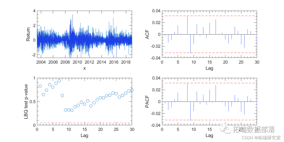

Figure 2. Return correlation test. The Ljung-Box Q test (bottom left) did not show significant serial autocorrelation as returns.

However, we can easily identify periods of clustering of absolute return values (regardless of the sign of the returns). Therefore, there is significant serial correlation in absolute return values.

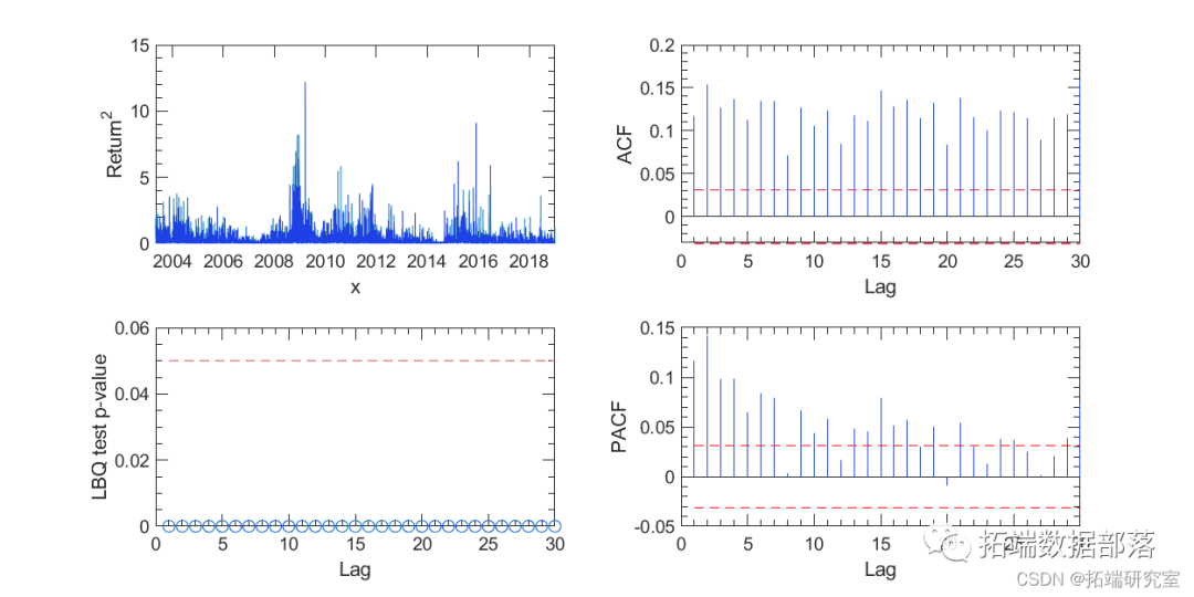
Figure 3. Correlation test of squared returns.

Click the title to view past content

R language modeling of financial time series data using multivariate ARMA, GARCH, EWMA, ETS, and Stochastic Volatility SV models

Swipe left to see more

01

02

03

04

GARCH (Generalized Autoregressive Conditional Heteroskedasticity) Model

The GARCH(1,1) model can be estimated using MATLAB’s Econometrics Toolbox. The ACF, PACF, and Ljung-Box Q tests in Figures 4 and 5 did not show significant serial correlation in the residuals and their squares. The residuals in the top left of Figure 4 visually resemble white noise rather than the original return series.

Mdls.dsVadjnce = garc(1,1);

[EsastMdl,EssddkjParamsCovf,lsdoggL,isdjngfo] = estimate(Msddl,rstan);

[Egf,hgV,logfgL] = inffgher(EstsdMdl,arstn);

gfh= Egh./sqrt(Vf);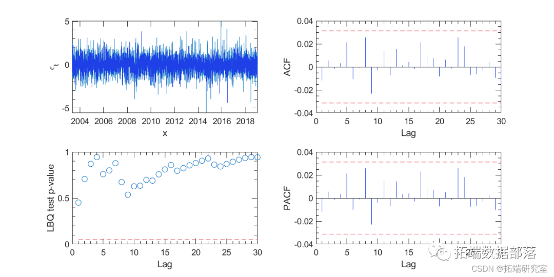

Figure 4. Correlation test of residuals from the GARCH(1,1) model.

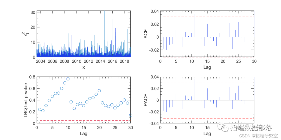
Figure 5. Correlation test of squared residuals from the GARCH(1,1) model.

plot(at,dad)set(gsdcaa);set(gasdca);ylabel('GARCH Volatility h_t');

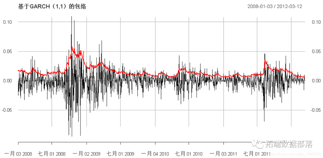
Figure 6. Volatility of the GARCH(1,1) model.

Markov Chain Monte Carlo (MCMC)

MCMC consists of two parts. The Monte Carlo part deals with how to draw random samples from a given probability distribution. The Markov chain part aims to generate a stable random process, known as a Markov process, so that the samples drawn sequentially through the Monte Carlo method approach those drawn from the “true” probability distribution.

We can then iteratively use the Gibbs sampling method to produce a series of parameters. Often discarded because it does nothing but normalize the distribution. The posterior distribution is incomplete. The Metropolis sampling method and the more general Metropolis-Hastings sampling method are used in this scenario. These two sampling methods are more commonly used for non-conjugate prior distributions where it is difficult to formulate a complete conditional posterior distribution.

% --- MCMC parameters

nmc = 10000;

bechvzta_mcmc = nan(nmc;dmc,1);

loxvgh_mcmc = nan(an,nmcjkldsmc);

alpha_mcmc = nan(nmcmssdc,length(alspdha0));

Sigmacvv_mcmc = nan(nmytsdcmc,1);


    % --- Gibbs sampling: beta    rtnas_new = rtn./sqdssrt(exp(logshis)); % Reformat return series    x = 1./sqrt(exp(lsogshisd));

    V_gfbeta = 1/(x'*x + 1/Sigsgfma_bdeta0);g

    E_bgexta = V_bfgetfga*(beta0/Sifgma_beta0+gdfxf'*rtndf_new);

    betxa = cnormrnd(E_beta,sqrt(fgV_bfdfgeta));

    % --- Metropolis sampling: ht    loghn1 = alphjklai(1)+alphai(2)*(alphai(1)+alphai(2)*loghi(n-1));

    loghf1 = [loghi(2:end); loghn1]; % Forward step ht's log    loghb1 = [logh0; loghi(1:end-1)]; % Backward step ht's log    % - Propose new ht    lojkghp = normrnd(lohghjkli,sijlgma_jlogjhp);

    % - Check the log ratio of posterior probability    logr = log(normpdf(loghp, [ones(n,1),loghb1]*alphai',sqrt(Sigmavi))) + ...


    % --- Gibbs sampling alpha    zasdt = [ones(n-1,1),lokkghi(1:end-1)];

    V_alpghas = inv( inv(Sigjkmahjg_alpjha0) + zt'*zt/Si;gmavkl;i);

    E_aldfhpha = V_alpha*(inv(Sigmjhja_abvnl;'lpha0)*akllpha0' + zt'*loghi(2:end)/Smavi);

    alvbphai = mvnrnd(E_vbal,npnha,V_bnm,bvalpha);

    % --- Gibbs sampling: Sigfmav    SfSR = sum((logfgjhi(2:ehgjnd)-zt*alphaighj').^2);

    % Alternative method for SSR via OLS    Sigjhavi = 1/randolhkm('Gamma',(nu0+n-1)/2,2/(nu0*Sigmavl;'k0+SSR));

Stochastic Volatility (SV) Model

Random modeling of volatility began in the early 1980s and became applicable after the paper by Jacquier, Polson, and Rossi provided clear evidence of stochastic volatility in 1994. The main difference between SV and GARCH models is the volatility innovation. In GARCH models, the time-varying volatility follows a deterministic process (there are no random terms in the volatility equation), while in SV models, it is random.

%% MCMC for Stochastic Volatility

% --- Prior parameters

Sigwertma_aelpha0 = etdiagweetwr([0.4,0.4]); % Covariance

% - For sigrmea^2_v

nu0 = 1;

Sigemav0 = 0.01;


% --- Using GARCH(1,1) model initial values, and least squares fit of log(ht0)

bewtwai = EstMtydl.rtyConrtystatynt;

MrgeyDL = etyrffitytlm();

alpefdgrtyhai = Mdl.Cvxoertyefficients{:,1}';

Sigretyrxmavi = nanvar(Mderyl.Reyefsidrdtyeruals.Raw);

However, obtaining a normalized factor for the approximate form of the probability distribution is not straightforward. We can use brute force calculations to generate a probability grid for each possible value and then draw from the grid. This is called the Griddy Gibbs method. Alternatively, we can use the Metropolis algorithm. In this algorithm, the proposal distribution from which to draw can be any symmetric distribution function. The proposal distribution function can also be asymmetric. But in this case, additional terms need to be included when calculating the probability ratio from jumping to balance this asymmetry. This is called the Metropolis-Hastings algorithm.

More complex proposal methods for the Metropolis-Hastings algorithm can be used to reduce correlation in the sequence, such as Hamiltonian MCMC.

subplot(4,1,1);plot(beasdta_mcmc);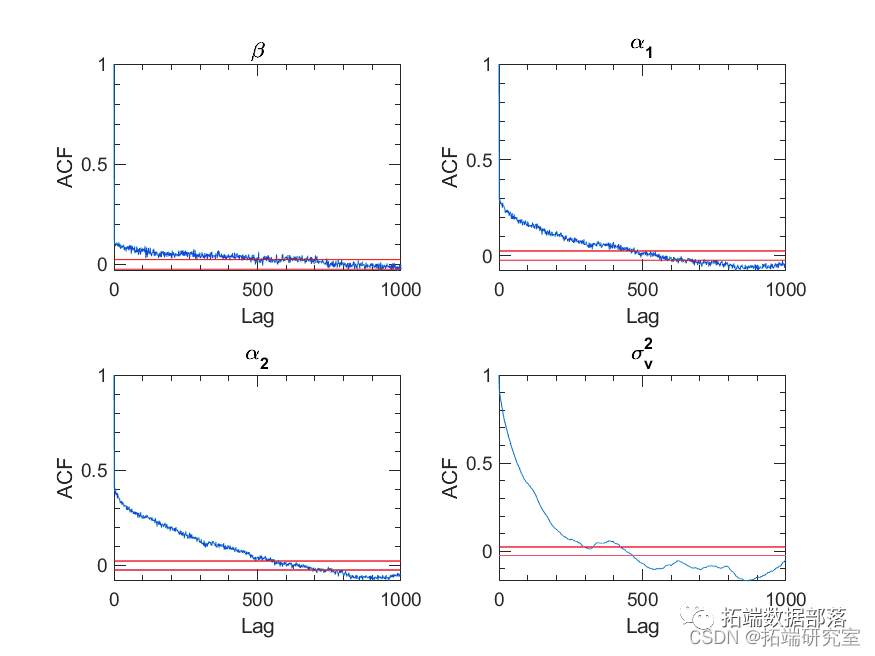

Figure 8. Autocorrelation of parameter sequences after burn-in. The red line indicates the 5% significance level.

Results and Discussion

After removing the burn-in, we obtain a set of parameter samples that can be approximately randomly drawn from the true high-dimensional joint distribution of the parameters. We can then perform statistical inference on these parameters. For example, the joint distribution of paired parameters and the marginal distribution of each parameter are shown in Figure 9. We can use the joint distribution to test this claim. Clearly, it is uncorrelated with the remaining parameters, as expected, and highly correlated, using their joint posterior distribution to demonstrate the reasonableness of the sampling. To improve sampling efficiency and reduce the correlation of samples in the sequence, we can sample from the above algorithm and from their trivariate joint posterior distribution. However, calculating a tight form of the posterior distribution for variables with different prior distributions is quite cumbersome, if not entirely impossible. In this case, the Metropolis-Hastings sampling method will certainly find its advantages.

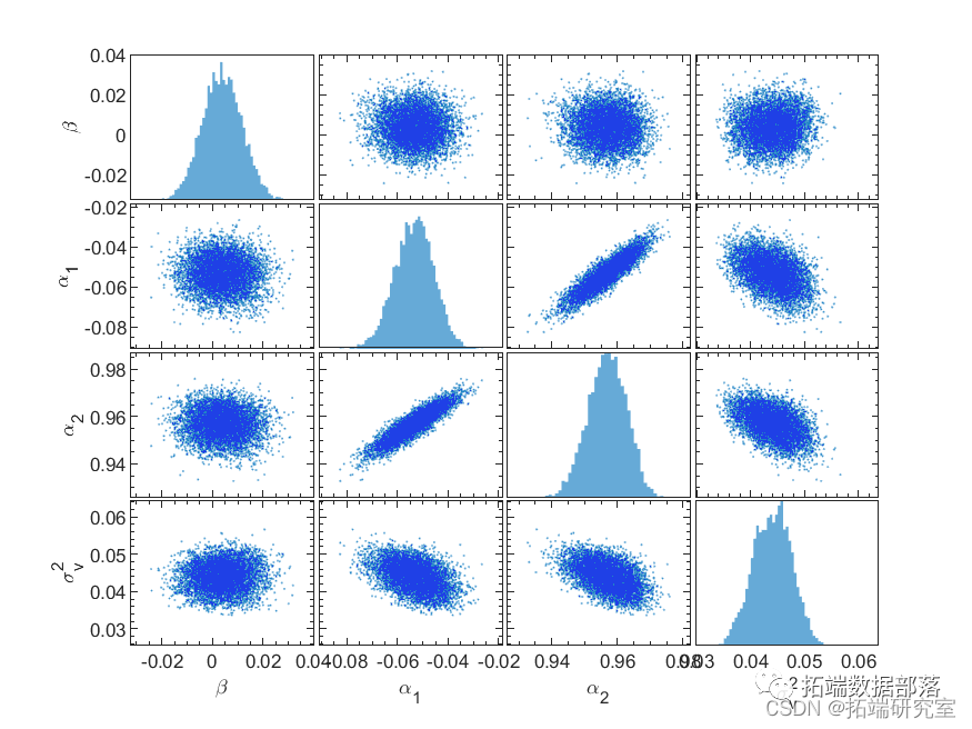
Figure 9. Scatter plot of the joint distribution of paired parameters (non-diagonal panels) and histograms of the marginal distributions of parameters (diagonal panels).

The stochastic volatility and its confidence bands are obtained by calculating the mean of the sampled volatility after the sequence stabilizes and the 2.5% and 97.5% quantiles. It is plotted in Figure 10.

h_mcmc = exp(logf_mds_mcmc);nbudrin = 4000;lb = quanile(h_mcd,bunn+1:end),0.025,2);   % 2.5% quantileub = quatgjeh_mcmc(nburhjkin+1:end)fhjk,0.975,2);   % 97.5% quantileholdghfd on; box on;plot(1:lengtgdhfh(t),V,'',dhfg1)plot(1:length(t),mdfghean(h_mcmc(:,nburnhgdf:enddgfh2),'linekljwdth',1)s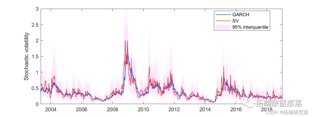

Figure 10. Posterior mean of stochastic volatility after 4000 burn-in iterations. The confidence bands for the stochastic volatility are shown in red for the 95% quantiles.

The stochastic volatility of the SV model is generally very similar to that of the GARCH model but is more erratic. This is natural because an additional random term is assumed in the SV model. The main advantage of using the stochastic volatility model compared to other models is that volatility is modeled as a random process rather than a deterministic process. This allows us to obtain an approximate distribution of volatility at each time in the sequence. When applied to volatility forecasting, stochastic models can provide confidence for predictions. On the other hand, the downsides are also evident. The computational cost is relatively high.

The data and code analyzed in this article are shared in the member group. Scan the QR code below to join the group!

Click at the end “Read the original”

to obtain the complete data.

This article is excerpted from “Analysis of Exchange Rate Time Series Using MCMC Markov Chain Monte Carlo Method for Stochastic Volatility SV and GARCH in MATLAB”.

Click the title to view past content

R language hidden Markov model HMM continuous sequence importance resampling CSIR estimation stochastic volatility model SV analysis of stock return time seriesMarkov regime switching model analysis of fund interest ratesMarkov regime switching modelTime-varying Markov regime switching MRS autoregressive model analysis of economic time seriesMarkov switching model study of traffic casualty accident time series forecastingHow to implement Markov Chain Monte Carlo MCMC models, Metropolis algorithm?Matlab using BUGS Markov regime switching random volatility model, sequential Monte Carlo SMC, M H sampling analysis of time seriesR language BUGS sequential Monte Carlo SMC, Markov switching stochastic volatility SV model, particle filtering, Metropolis Hasting sampling time series analysisMatlab using Markov Chain Monte Carlo (MCMC) logistic regression model analysis of automotive experimental dataStata Markov regime switching model analysis of fund interest ratesPYTHON using time-varying Markov regime switching (MRS) autoregressive model analysis of economic time seriesR language using Markov chains for channel attribution modeling in marketingMatlab implementing MCMC Markov switching ARMA – GARCH model estimationR language hidden Markov model HMM identification of changing stock market conditionsExamples of hidden Markov HMM models in RUsing machine learning to identify changing stock market conditions—hidden Markov model (HMM)Matlab Markov Chain Monte Carlo method (MCMC) estimation of stochastic volatility (SV) modelMarkov regime switching model in MATLABMatlab Markov regime switching dynamic regression model estimation of GDP growth rateR language Markov regime switching modelStata Markov regime switching model analysis of fund interest ratesR language how to do Markov switching modelR language hidden Markov model HMM identification of stock market change analysis reportImplementing Markov Chain Monte Carlo MCMC models in R