At this point, the matter should be settled, but I still have questions:
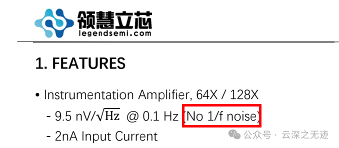
However, there is still a value at 0.1Hz. Is this a mistake?
What Does “No 1/f Noise” Really Mean?
It does not mean: noise = 0, or no low-frequency noise, or that low-frequency noise density approaches 0.
Rather, it means:
The input noise spectral density does not increase with frequency at low frequencies; there is no 1/f increase; that is, the noise spectrum is flat.
In other words:
The noise is white noise (flat noise), there is no 1/f corner frequency, and there is no typical pink noise bump caused by BJT/CMOS input stages.
Therefore:
“No 1/f noise” = this noise density is “flat” at low frequencies, not “zero”.
The white noise floor of the device can be:
9.5 nV/√Hz
12 nV/√Hz
30 nV/√Hz
… these are all “white noise” and not “1/f noise”.
Why Is There a Value at Low Frequency (0.1 Hz)?
To prove: that at 0.1 Hz, this extremely low frequency is still at the “white noise level”, without spiking (no pink noise).
Typical devices with 1/f noise will have noise densities at 0.1 Hz that become:
100 nV/√Hz
300 nV/√Hz
1 μV/√Hz
…
And chopper amplifiers (CHOP/Auto-zero) will shift the 1/f noise to high frequencies (modulation frequency), thus at DC, only the white noise floor remains; this is why at 0.1 Hz, the value is 9.5 nV/√Hz (almost the same as at mid-frequency).
How Can Chopper Amplifiers Achieve “No 1/f Noise”?
The chopper principle: modulates the input to tens of kHz (chopper frequency), amplifies at high frequency, and demodulates back to low frequency, moving all low-frequency noise (1/f) to high frequency (near the modulation frequency), with a low-pass filter at the output → all high-frequency noise is filtered out, leaving only white noise in the DC/low-frequency region.
Thus: at 0.1 Hz (even down to 10 mHz), no 1/f noise rise is observed, and the noise density is “flat (white) + extremely low”.
Does 9.5 nV/√Hz Mean “There Is Low-Frequency Noise”?
No. That is the white noise floor, not frequency-dependent noise.
What is observed is: the absolute size of the noise (white noise level), while 1/f noise refers to frequency-dependent noise.
For example:
| Noise Type | Does it Change with Frequency? | Example |
|---|---|---|
| White Noise (No 1/f) | Unchanged (flat) | 9.5 nV/√Hz @ 0.1 Hz, 1 Hz, 10 Hz… |
| 1/f Noise (Pink Noise) | Increases as f decreases | 100 nV/√Hz @1Hz, 1μV/√Hz @0.1Hz |
Chopper ADC / INA tells you:
“At low frequencies, there is only white noise, no 1/f noise component.”
Why Do Data Sheets Write Both “9.5 nV/√Hz @0.1Hz” & “No 1/f”?
This is to allow engineers to quickly confirm:
“What is the low-frequency noise density?” (absolute value)
“Is there 1/f?” (noise type)
So both lines must be viewed together for accuracy:
9.5 nV/√Hz → the white noise floor is very low
No 1/f → low-frequency noise does not increase with frequency
This is a characteristic that 24-bit ΔΣ ADCs must possess for measurement instruments, weighing, pressure sensors, etc.
“No 1/f” does not mean “noise=0”, but rather indicates “low-frequency noise remains at the white noise floor, not increasing with frequency”; 9.5 nV/√Hz is the value of the white noise floor, not 1/f noise; these two are completely non-contradictory.
Simulation
Frequency Spectrum: “With 1/f” vs “No 1/f (Chopper)”
Manually Set Theoretical Noise Spectrum
In the code, a theoretical ASD (Amplitude Spectral Density) is first created:
f = np.logspace(-3, 3, 1000)   # 1 mHz ~ 1 kHz
en_white = 10e-9               # 10 nV/√Hz white noise floor
fc = 1.0                        # 1 Hz corner frequency

# No 1/f: pure white noise
en_flat = en_white * np.ones_like(f)

# With 1/f: low frequency rises ~ sqrt(fc/f)
en_1f = en_white * np.sqrt(1 + fc / f)
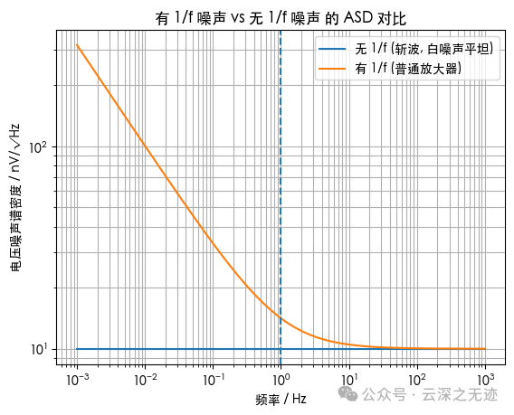
Blue line (No 1/f): remains at 10 nV/√Hz from 1 mHz to 1 kHz.
Orange line (With 1/f): at high frequencies (f ≫ 1Hz) ≈ 10 nV/√Hz; below 1Hz, it starts to rise, for example, at 0.01 Hz, it is about 10×, i.e., ≈ 100 nV/√Hz.
This graph is similar to what you see in operational amplifier datasheets:
Flat on the right, rising on the left → has 1/f;
Completely flat → chopper / Auto-zero / No 1/f.
The true meaning of “9.5 nV/√Hz @0.1Hz, No 1/f” is: at 0.1Hz, this extremely low frequency, the noise spectrum is STILL ≈ white noise floor, without rising.
Using Python to Generate a Segment of Noise with “1/f / No 1/f”
The previous graph was just a theoretical curve; next, I performed a more realistic simulation in the time domain.
First, Generate a Segment of White Noise
Fs = 1000.0       # Sampling rate 1 kS/s
T_total = 200.0   # Total duration 200 s
N = int(Fs * T_total)

np.random.seed(0)
x_white = np.random.normal(0, 1.0, N)   # Pure white noise
Shape the Noise in Frequency Domain to Create “With 1/f” Noise
Xw = np.fft.rfft(x_white)
freqs = np.fft.rfftfreq(N, d=1/Fs)
H_1f = np.sqrt(1 + fc / np.maximum(freqs, 1e-6))
H_1f[0] = 0.0  # Avoid infinity at DC
X_1f = Xw * H_1f
x_1f = np.fft.irfft(X_1f, n=N)
First, calculate the FFT of the white noise:<span>Xw</span>
Multiply by a shaping function<span>H_1f(f)=sqrt(1+fc/f)</span> → amplify low frequencies, keep high frequencies unchanged
Then IFFT back to the time domain: obtain <span>x_1f</span>, which is the noise with “1/f components”.
Then use the Welch method to estimate ASD:
freqs_est, asd_white = estimate_asd(x_white, Fs)
_, asd_1f_est = estimate_asd(x_1f, Fs)
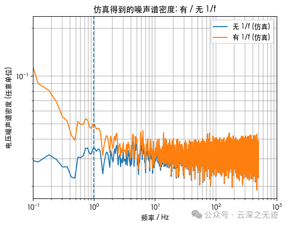
The second frequency spectrum graph (“simulated noise spectral density”) proves:
Blue line (x_white): spectrum is basically flat;
Orange line (x_1f): clearly rises below 1 Hz, consistent with the shape of 1/f.
This indicates that the time-domain random sequence we constructed indeed has the characteristics of “1/f noise”.
Why Is the RMS Noise of Chopper ADC Extremely Low Over 10 Seconds?
Method: RMS of “Averaged Values” at Different Averaging Times
We take two noise sequences <span>x_white</span> / <span>x_1f</span> and perform block averaging over different averaging times:
def rms_of_averaged(x, Fs, T_avg_list):
    rms_list = []
    for T in T_avg_list:
        L = int(T * Fs)                 # Number of samples per block
        nseg = len(x) // L
        segs = x[:nseg*L].reshape(nseg, L)
        means = segs.mean(axis=1)       # Average value of each block
        rms_list.append(np.sqrt(np.mean(means**2)))  # RMS of these average values
    return np.array(rms_list)

T_list = np.logspace(-1, 2, 20)  # 0.1s ~ 100s
rms_white = rms_of_averaged(x_white, Fs, T_list)
rms_1f = rms_of_averaged(x_1f, Fs, T_list)
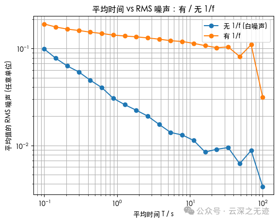
The final graph (Average Time vs RMS Noise) is very critical:
Horizontal axis: averaging time (0.1 s → 100 s, log scale)
Vertical axis: RMS of each block average value (log scale)
Blue line: No 1/f (white noise)
Orange line: With 1/f
From the graph, you can see:
White Noise (No 1/f):
The RMS noise decreases almost ideally; for example, from 0.1s → 10s, time ×100, RMS decreases by about /√100 = /10;
This is what you see in ΔΣ ADC datasheets:
“More averaging (more codes), lower ODR, noise decreases almost by bandwidth width reduction.”
In the context of ADC, this means: integrating for 10 seconds, the equivalent bandwidth is only a fraction of a Hz, and the white noise is averaged down very low, allowing you to see total RMS noise at the level of tens of nV.
With 1/f Noise:
Initially (T < 1s), the decreasing trend is good because the high-frequency part is still white noise; but when the averaging time extends to several seconds or tens of seconds, the curve clearly “flattens out”, no longer decreasing as quickly as 1/√T, and even tends towards a plateau; this is typical:
When low-frequency 1/f noise dominates, the longer the averaging time, the more you are just observing “long-term drift”, and the noise is not sufficiently averaged.
You can directly relate this to the “long-term drift of precision references / 1/f noise of operational amplifiers”: the longer you observe, the more you see slow drift, not random noise.
Translating Three Graphs Back to Your Concerned Chopper ADC Scenario
Frequency Spectrum:
Chopper ADC / INA: ASD is flat near DC → “No 1/f noise”.
Regular amplifiers: ASD rises below 1 Hz → “Has 1/f noise”.
Time Domain RMS Noise vs Averaging Time:
Chopper ADC: only white noise remains → averaging for 10 seconds, noise ~ original /√(10s·BW), can easily be reduced to tens of nV level.
Systems with 1/f: long-term averaging is limited by 1/f drift, and no matter how long you extend the time, it cannot be reduced further.
Combining CS5530 / LHA7530:
The datasheet states “9.5 nV/√Hz @0.1Hz, No 1/f noise”, which tells you: at low frequencies, there is only 9.5 nV/√Hz of white noise, with no additional 1/f “elevation”; thus, at 5~10 SPS (equivalent to bandwidth < 3 Hz), you can see extremely low RMS noise and 19~20 bit noise-free resolution, which is a natural mathematical result, not “magic”.
import numpy as np
import matplotlib.pyplot as plt

# =========================
# 1. Frequency Spectrum Comparison: With 1/f vs No 1/f
# =========================

# Frequency axis: 1e-3 Hz ~ 10^3 Hz
f = np.logspace(-3, 3, 1000)
en_white = 10e-9   # White noise floor 10 nV/√Hz
fc = 1.0           # 1/f corner frequency 1 Hz

# No 1/f: pure white noise
en_flat = en_white * np.ones_like(f)

# With 1/f: rises below fc ~ sqrt(fc/f)
en_1f = en_white * np.sqrt(1 + fc / f)

plt.figure()
plt.loglog(f, en_flat*1e9, label="No 1/f (Chopper, white noise flat)")
plt.loglog(f, en_1f*1e9, label="With 1/f (Regular amplifier)")
plt.axvline(fc, linestyle="--")
plt.xlabel("Frequency / Hz")
plt.ylabel("Voltage Noise Spectral Density / nV/√Hz")
plt.title("Comparison of ASD: With 1/f Noise vs No 1/f Noise")
plt.legend()
plt.grid(True, which="both")

# =========================
# 2. Time Domain Simulation: RMS Noise at 10s Averaging
# =========================

Fs = 1000.0          # Sampling rate 1 kS/s
T_total = 200.0      # Total duration 200 s
N = int(Fs * T_total)

# Generate a segment of white noise
np.random.seed(0)
x_white = np.random.normal(0, 1.0, N)

# Generate "With 1/f" noise through frequency domain shaping
Xw = np.fft.rfft(x_white)
freqs = np.fft.rfftfreq(N, d=1/Fs)
H_1f = np.sqrt(1 + fc / np.maximum(freqs, 1e-6))
H_1f[0] = 0.0  # Set DC component to 0 to avoid divergence
X_1f = Xw * H_1f
x_1f = np.fft.irfft(X_1f, n=N)

# Validate frequency spectrum: estimate ASD of both noise types
def estimate_asd(x, Fs, nfft=16384):
    w = np.hanning(nfft)
    step = nfft // 2
    segs = (len(x) - nfft) // step
    psd = np.zeros(nfft//2 + 1)
    for i in range(segs):
        seg = x[i*step:i*step+nfft] * w
        X = np.fft.rfft(seg)
        psd += (np.abs(X)**2) / (Fs * np.sum(w**2))
    psd /= segs
    freqs = np.fft.rfftfreq(nfft, d=1/Fs)
    asd = np.sqrt(psd)
    return freqs, asd

freqs_est, asd_white = estimate_asd(x_white, Fs)
_, asd_1f_est = estimate_asd(x_1f, Fs)

plt.figure()
plt.loglog(freqs_est[1:], asd_white[1:], label="No 1/f (Simulation)")
plt.loglog(freqs_est[1:], asd_1f_est[1:], label="With 1/f (Simulation)")
plt.axvline(fc, linestyle="--")
plt.xlim(1e-1, 1e3)
plt.xlabel("Frequency / Hz")
plt.ylabel("Voltage Noise Spectral Density (Arbitrary Units)")
plt.title("Simulated Noise Spectral Density: With / No 1/f")
plt.legend()
plt.grid(True, which="both")

# =========================
# 3. Statistical Average Time vs RMS Noise
# =========================

def rms_of_averaged(x, Fs, T_avg_list):
    rms_list = []
    for T in T_avg_list:
        L = int(T * Fs)
        nseg = len(x) // L
        if nseg == 0:
            rms_list.append(np.nan)
            continue
        segs = x[:nseg*L].reshape(nseg, L)
        means = segs.mean(axis=1)
        rms_list.append(np.sqrt(np.mean(means**2)))
    return np.array(rms_list)

T_list = np.logspace(-1, 2, 20)  # 0.1 s ~ 100 s
rms_white = rms_of_averaged(x_white, Fs, T_list)
rms_1f = rms_of_averaged(x_1f, Fs, T_list)

plt.figure()
plt.loglog(T_list, rms_white, 'o-', label="No 1/f (White Noise)")
plt.loglog(T_list, rms_1f, 'o-', label="With 1/f")
plt.xlabel("Averaging Time T / s")
plt.ylabel("RMS Noise of Average Values (Arbitrary Units)")
plt.title("Average Time vs RMS Noise: With / No 1/f")
plt.grid(True, which="both")
plt.legend()
plt.show()