Click on “Mathematics for Graduate Entrance Exams”↑ to gain knowledge every day!
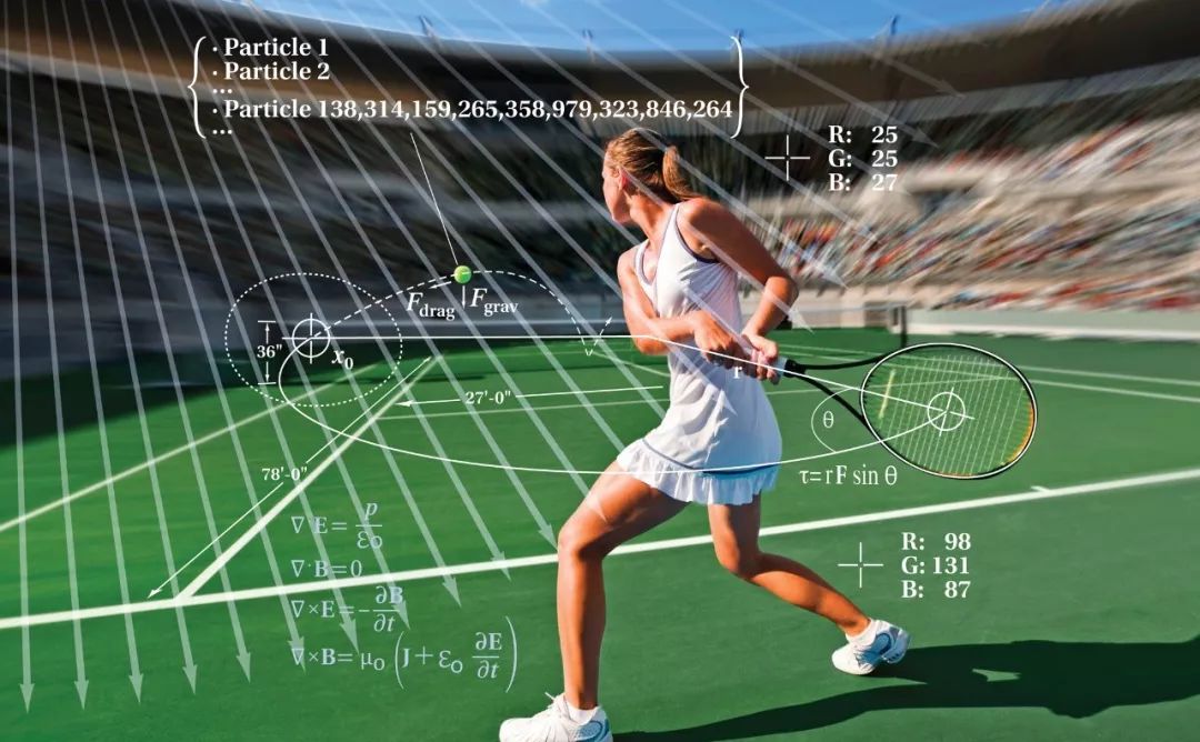
Illustration Source: discovermagazine.com
Article Source: Mathematics China (ID:shuxuezhongguo)
The National College Student Mathematical Modeling Competition has a long history and attracts students from all over the country to participate. Mastering certain modeling methods helps students perform better in the competition and increases the chances of winning.
Common methods used in mathematical modeling include: analogy method, bisection method, dimensional analysis, difference method, variational method, graph theory method, analytic hierarchy process, data fitting method, regression analysis, mathematical programming (linear programming, nonlinear programming, integer programming, dynamic programming, goal programming), mechanism analysis, queuing methods, game theory methods, decision-making methods, fuzzy evaluation methods, time series methods, gray theory methods, and modern optimization algorithms (tabu search algorithm, simulated annealing algorithm, genetic algorithm, neural networks).
These methods can solve the following models: optimization models, differential equation models, statistical models, probability models, graph theory models, decision models.
Fitting and interpolation methods (given a set of data points, determine a curve or surface that meets specific requirements to reflect the overall trend of the object): MATLAB can implement fitting for univariate functions, including polynomial and nonlinear functions, as well as multivariate function fitting, i.e., regression analysis, to determine functions; it can also implement piecewise linear, polynomial, spline, and multidimensional interpolation using MATLAB.
In optimization methods, decision variables, objective functions (as simple and smooth as possible), constraints, and solution methods are the four key factors. This includes unconstrained rules (implemented using fminsearch, fminbnd), linear rules (implemented using linprog), nonlinear rules (implemented using fmincon), multi-objective programming (with objective weighting, utility functions), dynamic programming (backward and forward), and integer programming.
Regression analysis: a statistical method used to approximate the average change relationship between variables based on the relationship shape of phenomena with relevant relationships (univariate linear regression, multivariate linear regression, nonlinear regression). Regression analysis studies several issues based on a set of data: establishing a regression model between the dependent variable and independent variables (empirical formulas); testing the credibility of the regression model; determining whether each independent variable significantly affects the dependent variable; assessing whether the regression model fits this set of data; and using the regression model for forecasting or control. Correspondingly, there are linear regression, multivariate polynomial regression, and nonlinear regression.
Stepwise regression analysis: starts with one independent variable and sequentially introduces independent variables into the regression equation based on their significance level: when an introduced independent variable becomes insignificant due to the introduction of later variables, it should be removed; introducing or removing an independent variable from the regression equation constitutes one step of stepwise regression; each step must undergo significance testing to ensure that only significant variables are included in the regression equation before introducing new significant variables; this process is repeated until no insignificant variables can be removed from the regression equation, and no significant variables can be introduced into the regression equation.
Cluster analysis: when there exists varying degrees of similarity between the studied samples or variables, it is necessary to find statistical measures that can quantify their similarity as the basis for classification, and then use these measures to classify the samples or variables.
Hierarchical cluster analysis— considers n samples or n indicators as n classes, where each class includes one sample or indicator, and then merges the two most similar classes into a new class, and so on. Ultimately, the number of classes can be determined based on needs, and how many samples (indicators) are included in each class.
Steps of the hierarchical clustering method:
1. Calculate the pairwise distances between n samples
2. Form n classes, each containing only one sample
3. Merge the two closest classes into a new class
4. Calculate the distance from the new class to the current classes (the distance from the new class to the current class equals the minimum distance between the current class and the classes contained in the merged class); if the number of classes equals 1, proceed to 5, otherwise return to 3
5. Draw the clustering diagram
6. Determine the number of classes and the classes.
Discriminant analysis: when the research objects are known to be divided into several types, and a batch of known samples of various types has been obtained, a discriminant function is established based on certain criteria, and then unknown type samples are classified.
Distance discriminant method— first calculates the centroids of each class based on known classified data, calculates the distance from new individuals to each class, and determines the shortest distance (Euclidean distance, Mahalanobis distance).
Fisher discriminant method— constructs a discriminant function using indicators of known category individuals (similar categories have small differences, different categories have large differences), and judges the category of new individuals based on the value of the discriminant function.
Bayes discriminant method— calculates the conditional probabilities of new samples belonging to each population, compares the probabilities, and assigns the new sample to the population with the highest probability.
Fuzzy mathematics: a branch of mathematics that studies and processes fuzzy phenomena (where there is no clear boundary between concepts and their opposites) and related issues: fuzzy classification problems—when several fuzzy concepts that are not clearly defined need to be evaluated against a certain definite object to determine which fuzzy concept reflects it more reasonably and accurately; fuzzy similarity selection—ordering a group of objects based on certain properties is a common problem, but the properties used for comparison have fuzzy boundaries; fuzzy cluster analysis—constructing a fuzzy matrix based on the inherent attributes of the research objects, and determining their classification relationships based on certain membership degrees; fuzzy analytic hierarchy process—determining pairwise comparison indicators; fuzzy comprehensive evaluation—making an overall evaluation of objects constrained by multiple factors, such as product quality assessment, scientific and technological achievement appraisal, or evaluating the adaptability of a certain crop for planting, all belong to comprehensive evaluation problems. Since evaluating objects from multiple perspectives inevitably involves fuzziness and subjectivity, using fuzzy mathematics for comprehensive evaluation will make the results as objective as possible, thus achieving better practical effects.
Time series refers to a sequence of data arranged in chronological order, which changes over time and is interrelated—by processing the time series of the forecast target itself, its change trend can be studied (long-term trend changes, seasonal changes, cyclical changes, irregular changes).
Autoregressive model: general autoregressive model AR(n)— the response of the system at time t is only related to its previous responses X(t) and not to disturbances that entered the system at previous times;
Moving average model MA(m)— the response of the system at time t is unrelated to its previous responses, but there is a certain correlation with disturbances that entered the system at previous times a(t-1),…,a(t-m);
Autoregressive moving average model ARMA(n,m)— the response of the system at time t is related not only to its previous n responses but also to disturbances that entered the system at previous m times.
Basic steps of time series modeling
1. Data preprocessing: removing and extracting trend items from data
2. Set n=1, fit the ARMA(2n,2n-1) (i.e., ARMA(2,1)) model
3. n=n+1, fit the ARMA(2n,2n-1) model
4. Use the F criterion to test the applicability of the model. If the test is significant, proceed to step 2. If the test is not significant, proceed to step 5.
5. Check whether the coefficient values of distant moments are very small and whether their confidence intervals contain zero. If not, the applicable model is ARMA(2n,2n-1). If very small and its confidence interval contains zero, fit ARMA(2n-1,2n-2).
6. Use the F criterion to test the models ARMA(2n,2n-1) and ARMA(2n-1,2n-2); if the F value is not significant, proceed to step 7; if the F value is significant, proceed to step 8.
7. Discard small MA parameters, fit the model ARMA(2n-1,m) with m<2n-2, and test using the F criterion. Repeat this process until the applicable model with the minimum parameters is obtained.
8. Discard small MA parameters, fit the model ARMA(2n,m) with m<2n-1, and test using the F criterion. Repeat this process until the applicable model with the minimum parameters is obtained.
Graph theory methods:
The shortest path problem: finding the shortest path between two specified vertices—given a railway network connecting several towns, find the shortest railway route between two specified towns (using Dijkstra’s algorithm) for the shortest path between each pair of vertices (using Dijkstra’s algorithm and Floyd’s algorithm).
The minimum spanning tree problem: connection problem—design a route map to construct a railway connecting multiple cities with the lowest total cost (using Prim’s algorithm and Kruskal’s algorithm).
The matching problem in graphs: personnel assignment problem: n workers are to do n jobs, where each person is suitable for one or several jobs. Can each person have a suitable job? If not, how many people can have suitable jobs at most? (using the Hungarian algorithm).
Traversal problem: the Chinese postman problem—when the postman delivers mail, he must start from the post office, travel through every street in his delivery area at least once, and then return to the post office, but he hopes to choose the shortest route.
Maximum flow problem.
Transportation problems:
Minimum cost maximum flow problem: in transportation problems, people always seek to find a transportation scheme that minimizes total transportation costs while completing transportation tasks.
Common algorithms used in mathematical modeling:
1: Monte Carlo algorithm;
2: Data fitting, parameter estimation, interpolation, and other data processing algorithms (commonly implemented using MATLAB);
3: Linear programming, integer programming, multivariate programming, quadratic programming (can be implemented using LINGO, LINGO, MATLAB);
4: Graph theory algorithms (including shortest path, network flow, bipartite graphs);
5: Dynamic programming, backtracking search, divide and conquer algorithms, branch and bound;
6: Three classic algorithms of optimization theory (simulated annealing algorithm, neural network algorithm, genetic algorithm);
7: Grid algorithms and exhaustive methods;
8: Continuous data discretization;
9: Numerical analysis algorithms;
10: Image processing algorithms (commonly implemented using MATLAB).
Disclaimer: The content sources are indicated, and reprints are for learning and communication purposes only. If the original source disagrees with the reprint, please contact us for deletion. Thank you!The shared content is for reflection only and does not represent the views of this account!

↓↓↓ Click to read the original text for more related content