Author Introduction

snowwave02
PhD, Senior Engineer
Team snowwave02: A software development team in the field of design simulation, composed of professionals in software, mechanics, physics, etc., with over 10 years of CAD/CAE software development experience, proficient in Abaqus secondary development, having undertaken multiple large design simulation projects in aerospace, aviation, shipping, and machinery industries, with rich practical experience.At the end of this article, a free video tutorial titled “Basic Theory -> Abaqus Operation -> MATLAB Programming” by the author’s team is attached, explaining the implementation of linear strain in commercial software or self-developed software within elements.This article is originally published by the author on the Technical Neighbor platform, and reprinting requires author authorization.
Overview
This series of articles studies the mature basic theory of finite elements and its implementation methods in commercial finite element software.The theory of finite elements has developed over several decades and is quite mature; commercial finite element software also adopts these mature finite element theories, but in practical applications, commercial CAE software makes corresponding corrections based on traditional theoretical foundations to solve different problems encountered in engineering, and each software has different correction methods. Each mainstream commercial software manual indicates which theoretical formulas are adopted for each element, but only briefly mentions the methods of correction, with many lacking specific implementation formulas.Commercial software is essentially a black box; except for developers, users can only guess the internal implementation methods from outside the black box.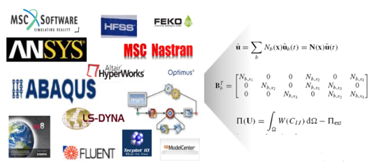 On one hand, we refer to the theoretical manuals of various mainstream commercial software and guess the internal correction methods through extensive data research; on the other hand, we develop our own structural finite element solver through programming, verifying our guesses by comparing the results of our self-developed solver with those of commercial software, akin to peering through a tube to study correction methods, thereby inferring the internal computational methods of commercial finite element software.We focus on structural finite elements in CAE, so we primarily chose Abaqus, which has relatively complete documentation among commercial structural finite element software, to study its internal implementation methods. We will also touch on other commercial software like Nastran/Ansys for certain issues. For ease of understanding, many problems are mathematically not rigorous, and due to limited expertise, there may be many theoretical errors. We welcome discussions and look forward to more collaboration opportunities.iSolver Introduction Video(Copy the link to your browser to open)::http://www.jishulink.com/college/video/c12884
Difference Between Explicit and Implicit Methods
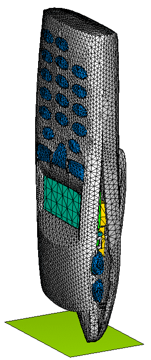
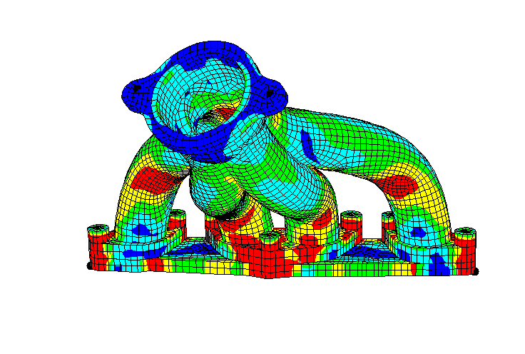
There are generally two types of CAE solving methods: Explicit and Implicit. The explicit solving algorithm is based on dynamic equations, where the displacement at the current moment is only related to the velocity and displacement at the previous moment, and no iteration is required during the solving process; while the implicit solving is based on the principle of virtual work, which generally requires iterative calculations.In Abaqus, both explicit and implicit solvers typically employ incremental solving, dividing the analysis step into several incremental steps, calculating the next incremental step when equilibrium is reached in the current incremental step.1. ExplicitIn the explicit solving process, no iterative solving is needed within each incremental step, and there is no need to form a tangent stiffness matrix, so the computational load within each incremental step is relatively small, generally proportional to the element size. However, the incremental step length cannot be too large, generally not exceeding 1/10 of the model’s minimum natural oscillation period, otherwise it may lead to divergence in the results.

2. ImplicitIn the implicit solving process, each incremental step requires balancing iterations and forming a tangent stiffness matrix, resulting in a relatively large computational load, generally related to the element size and the convergence speed of iterations. The convergence speed and stability of implicit solving vary based on the chosen iterative methods. Therefore, it is necessary to select an appropriate incremental step length based on the model characteristics to ensure convergence of the results.
In summary, whether explicit or implicit solving, it is crucial to reasonably set the incremental step length and solving method based on the model and solving problem to ensure the accuracy and quality of the analysis. Although these two solving methods are already basic dynamic solving methods in finite elements, due to the complexity of finite elements themselves, many people often find it difficult to understand the differences between the two and why explicit methods diverge. This article will use a simple example along with code implementation to intuitively explain the differences between implicit and explicit methods.
1.1 Forward Euler and Backward Euler
Forward Euler and Backward Euler are typical computational methods for explicit and implicit solving, respectively. This article will reference these two methods to intuitively demonstrate the differences between explicit and implicit solving.Forward Euler:fn+1 (x) = fn (x) + h*f’n (x)Backward Euler:fn+1 (x) = fn (x) + h*f’n+1 (x)
1.2 Example
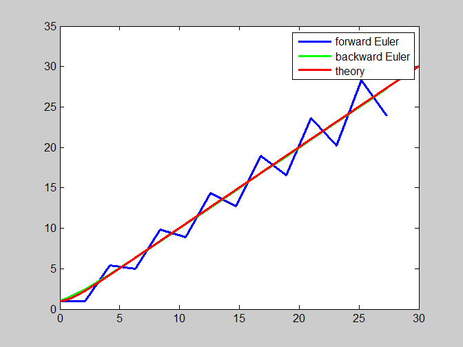
Now, let’s take a differential equation as an example:y'(x) = -y+x+1with y(0) = 1.1. Forward Euler MethodUsing the Forward Euler method, we get:yn+1 = yn + h*(-yn + xn + 1)Clearly, this equation requires no additional calculations to derive yn+1 from yn, thus each iterative computation is small. However, h has a maximum limit, as detailed in the derivation process below:yn+1 = (1-h)yn + h*(xn + 1)We can derive:yn+1 = (1-h)2 yn-1 + h*(xn + 1) + h*(xn-1 + 1)Thus, we find:yn+1 = (1-h)n + O(s2)When h < 2, y converges, but when h >= 2, y diverges.2. Backward Euler Methodyn+1 = yn + h*(-yn+1 + xn+1 + 1)This equation cannot directly yield yn+1; further calculations are needed to obtain:yn+1 = (yn + h*(xn+1 + 1)) / (1+h)When h > 0, y converges unconditionally.3. Result ComparisonAssuming n = 30(1) When h = 1.9, the calculation results are shown in the following figures, both explicit and implicit are close to the theoretical results: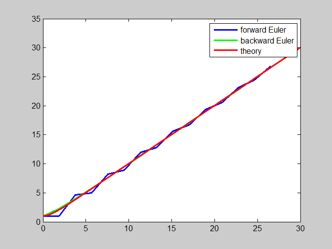 (2) When h = 2.1, the calculation results are shown in the following figures, and the explicit solving diverged:
Conclusion
This article briefly introduces the differences between explicit and implicit methods, which essentially arise from the use of different physical balance equations, thus exhibiting different behaviors in various physical problems. The article provides a mathematical example and solves it using both Forward Euler and Backward Euler methods to intuitively demonstrate the differences between explicit and implicit methods in the solving process, as well as the impact of incremental step length on the results.
If you have any other questions or project collaboration intentions, feel free to message us on Technical Neighbor.To obtain the <MATLAB code for explicit and implicit methods mentioned in the article>, please click to read the original text.
High-Quality Free Course
“In-Depth Finite Element Analysis: Basic Theory -> Abaqus Operation -> MATLAB Programming”

(1) Course IntroductionThe course on finite elements adopts:1. PPT-based theoretical explanations2. Demonstrations of Abaqus software operations3. MATLAB programming demonstrations and hands-on practice for studentsThe combination of these three approaches helps everyone get started with complex and tedious structural finite elements in a simple and intuitive way, while also diving into the programming level to understand the theoretical and internal implementation principles of commercial software.(2) Suitable AudienceThis may be useful for the following four types of personnel:1. Beginners who do not understand finite element theory well and find the formulas in books too complex to comprehend.2. Explorers who are not satisfied with merely operating commercial CAE software but wish to understand the internal implementation of finite element software.3. Pioneers of domestic independent industrial software who seek to develop autonomous CAE software but do not know where to start from scratch.4. Application engineers in the CAE field who wish to implement custom elements, materials, etc., in practical engineering.(3) Tool DownloadThe self-developed finite element solver development platform iSolver is required in the video, download (copy to your browser):http://www.jishulink.com/content/post/337351(4) Main ContentPart One: 01. General Introduction1. Course objectives and introduction2. Brief discussion on static and modal analysis3. Finite element approximation and incremental iterative method process4. Implementation of the simplest shell element in two lines of codePart Two: 02. S4R Stretching Example:1. Virtual work principle, derivation of general element stiffness matrix, classification of shell elements, isoparametric space2. Steps for shell element membrane stiffness algorithm3. MATLAB programming step-by-step demonstration4. Principle analysisPart Three: 03. Software Introduction1. Introduction to commercial structural finite element software Abaqus2. Introduction to self-developed finite element development platform iSolverPart Four: 04. S4 In-Plane Bending ExamplePart Five: 05. S4 Modal Analysis ExamplePart Six: 06. Improvements and PracticeWith limited expertise, if this video helps you in any way, we will be very pleased.At the same time, we welcome comments and discussions, constructive criticism, and look forward to more collaboration opportunities; you can message our team on Technical Neighbor.“Series of Free Courses”
-END-
 Click to read the original text to obtain the code!