
Introduction: Recently, I have been working on data processing related to acceleration, needing to integrate acceleration into displacement. I found that there isn’t much information available online, so I will summarize what I have done recently!
There are mainly two methods for integration: time-domain integration and frequency-domain integration. A common issue with integration is the generation of a secondary trend. Regarding the methods of integration, someone in a foreign forum proposed the following for reference.

Double integration of raw acceleration data is a pretty poor estimate for displacement. The reason is that at each integration, you are compounding the noise in the data.
If you are dead set on working in the time-domain, the best results come from the following steps.
-
Remove the mean from your sample (now have zero-mean sample)
-
Integrate once to get velocity using some rule (trapezoidal, etc.)
-
Remove the mean from the velocity
-
Integrate again to get displacement.
-
Remove the mean. Note, if you plot this, you will see drift over time.
-
To eliminate (some to most) of the drift (trend), use a least squares fit (high degree depending on data) to determine polynomial coefficients.
-
Remove the least squares polynomial function from your data.
A much better way to get displacement from acceleration data is to work in the frequency domain. To do this, follow these steps…
-
Remove the mean from the acceleration data
-
Take the Fourier transform (FFT) of the acceleration data.
-
Convert the transformed acceleration data to displacement data by dividing each element by -omega^2, where omega is the frequency band.
-
Now take the inverse FFT to get back to the time-domain and scale your result.
This will give you a much better estimate of displacement.

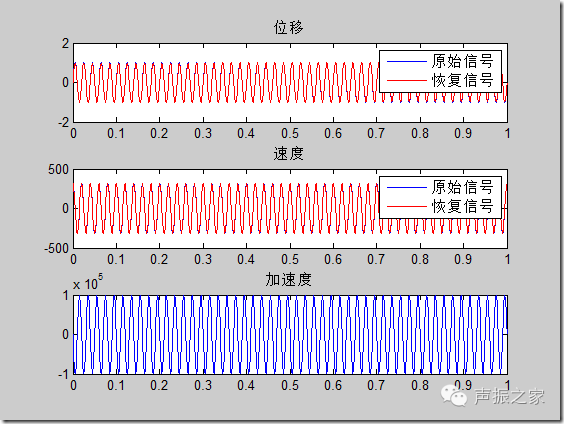
In the end, frequency-domain integration is more effective than time-domain integration, which has also been confirmed by practical tests. The reason may be that during time-domain integration, removing the trend reduces the energy of the signal, so the final result often appears smaller than the actual amplitude. Below are some tests where I performed double integration on a sine signal with a frequency of 50Hz and a sampling frequency of 1000Hz, with the recovery results shown below:
Time-Domain Integration
Frequency-Domain Integration
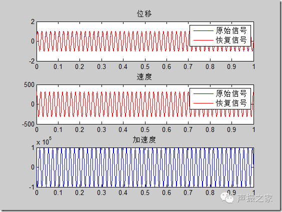
It can be seen that the recovery signals are good (for 50Hz, this is the effect).
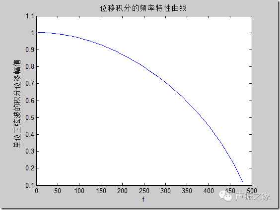
The frequency characteristic curves of the two methods are analyzed as follows:
Time-Domain Integration
Frequency-Domain Integration
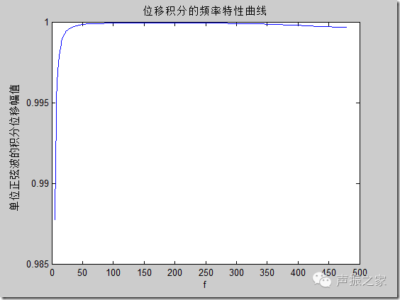
It can be seen that frequency-domain integration yields better signals, while time-domain integration shows a decrease in the recovered sine amplitude as the signal frequency increases.
For signals containing two sine waves, frequency-domain integration recovers the signal normally, while time-domain integration has errors in recovering high-frequency information; for noisy sine signals, noise can cause the integration results to produce large trend terms (not just simple secondary trends), as shown in the figure below:
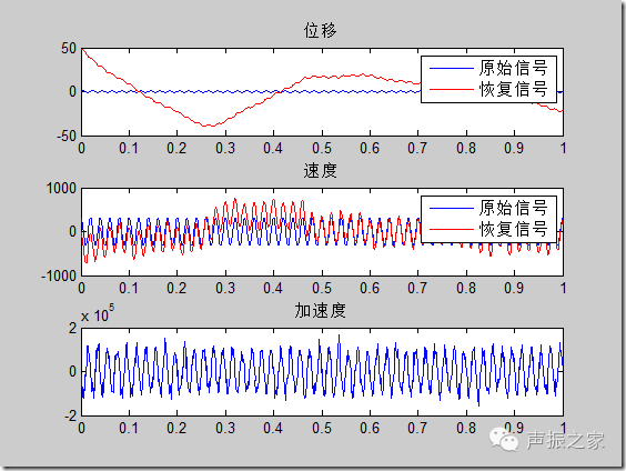
In this case, filtering methods can be used to remove the large trend terms.
The test code is as follows:
% Test the effect of integration on sine signals
clc
clear
close all
%% Original Sine Signal
ts = 0.001;
fs = 1/ts;
t = 0:ts:1000*ts;
f = 50;
dis = sin(2*pi*f*t);
% Displacement
vel = 2*pi*f.*cos(2*pi*f*t);
% Velocity
acc = -(2*pi*f).^2.*sin(2*pi*f*t);
% Acceleration
% Test with multiple sine waves
% f1 = 400;
% dis1 = sin(2*pi*f1*t); % Displacement
% vel1 = 2*pi*f1.*cos(2*pi*f1*t); % Velocity
% acc1 = -(2*pi*f1).^2.*sin(2*pi*f1*t); % Acceleration
% dis = dis + dis1;
% vel = vel + vel1;
% acc = acc + acc1;
% Conclusion: frequency-domain integration recovers the signal normally, while time-domain integration has errors in recovering added high-frequency information
% Noise test
acc = acc + (2*pi*f).^2*0.2*randn(size(acc));
% Conclusion: noise can cause large trend terms in the integration results
figure
ax(1) = subplot(311);
plot(t, dis), title(‘Displacement’)
ax(2) = subplot(312);
plot(t, vel), title(‘Velocity’)
ax(3) = subplot(313);
plot(t, acc), title(‘Acceleration’)
linkaxes(ax, ‘x’);
% Calculate displacement from acceleration signal
[disint, velint] = IntFcn(acc, t, ts, 2);
axes(ax(2));
hold on
plot(t, velint, ‘r’),
legend({‘Original Signal’, ‘Recovered Signal’})
axes(ax(1));
hold on
plot(t, disint, ‘r’),
legend({‘Original Signal’, ‘Recovered Signal’})
%% Test the frequency characteristics of the integration operator
n = 30;
amp = zeros(n, 1);
f = [5:30 40:10:480];
figure
for i = 1:length(f)
fi = f(i);
acc = -(2*pi*fi).^2.*sin(2*pi*fi*t);
% Acceleration
[disint, velint] = IntFcn(acc, t, ts, 2);
% Integrate to get displacement
amp(i) = sqrt(sum(disint.^2))/sqrt(sum(dis.^2));
plot(t, disint)
drawnow
%pause
end
close
figure
plot(f, amp)
title(‘Frequency Characteristics Curve of Displacement Integration’)
xlabel(‘f’)
ylabel(‘Amplitude of Integrated Displacement of Unit Sine Wave’)
The code above uses the IntFcn function to perform integration, which is a wrapped function that can perform both time-domain and frequency-domain integration. Its code is as follows:
% The integration operation calculates displacement from acceleration, with options for time-domain and frequency-domain integration
function [disint, velint] = IntFcn(acc, t, ts, flag)
if flag == 1
% Time-Domain Integration
[disint, velint] = IntFcn_Time(t, acc);
velenergy = sqrt(sum(velint.^2));
velint = detrend(velint);
velreenergy = sqrt(sum(velint.^2));
velint = velint/velreenergy*velenergy;
disenergy = sqrt(sum(disint.^2));
disint = detrend(disint);
disreenergy = sqrt(sum(disint.^2));
disint = disint/disreenergy*disenergy;
% This operation is to compensate for the energy loss during trend removal
% Remove the quadratic term from displacement
p = polyfit(t, disint, 2);
disint = disint – polyval(p, t);
else
% Frequency-Domain Integration
velint = iomega(acc, ts, 3, 2);
velint = detrend(velint);
disint = iomega(acc, ts, 3, 1);
% Remove the quadratic term from displacement
p = polyfit(t, disint, 2);
disint = disint – polyval(p, t);
end
end
The sub-function for time-domain integration is as follows:
% Time-domain trapezoidal integration
function [xn, vn] = IntFcn_Time(t, an)
vn = cumtrapz(t, an);
vn = vn – repmat(mean(vn), size(vn,1), 1);
xn = cumtrapz(t, vn);
xn = xn – repmat(mean(xn), size(xn,1), 1);
end
The sub-function for frequency-domain integration is as follows (this code was written by a foreigner, implementing integration and differentiation operations in the frequency domain)
function dataout = iomega(datain, dt, datain_type, dataout_type)
%%%%%%%%%%%%%
%
% IOMEGA is a MATLAB script for converting displacement, velocity, or
% acceleration time-series to either displacement, velocity, or
% acceleration times-series. The script takes an array of waveform data
% (datain), transforms into the frequency-domain in order to more easily
% convert into desired output form, and then converts back into the time
% domain resulting in output (dataout) that is converted into the desired
% form.
%
% Variables:
% ———-
%
% datain = input waveform data of type datain_type
%
% dataout = output waveform data of type dataout_type
%
% dt = time increment (units of seconds per sample)
%
% 1 – Displacement
% datain_type = 2 – Velocity
% 3 – Acceleration
%
% 1 – Displacement
% dataout_type = 2 – Velocity
% 3 – Acceleration
%
%%%%%%%%%%%%%
% Make sure that datain_type and dataout_type are either 1, 2 or 3
if (datain_type < 1 || datain_type > 3)
error(‘Value for datain_type must be a 1, 2 or 3’);
elseif (dataout_type < 1 || dataout_type > 3)
error(‘Value for dataout_type must be a 1, 2 or 3’);
end
% Determine Number of points (next power of 2), frequency increment
% and Nyquist frequency
N = 2^nextpow2(max(size(datain)));
df = 1/(N*dt);
Nyq = 1/(2*dt);
% Save frequency array
iomega_array = 1i*2*pi*(-Nyq : df : Nyq-df);
iomega_exp = dataout_type – datain_type;
% Pad datain array with zeros (if needed)
size1 = size(datain,1);
size2 = size(datain,2);
if (N-size1 ~= 0 && N-size2 ~= 0)
if size1 > size2
datain = vertcat(datain,zeros(N-size1,1));
else
datain = horzcat(datain,zeros(1,N-size2));
end
end
% Transform datain into frequency domain via FFT and shift output (A)
% so that zero-frequency amplitude is in the middle of the array
% (instead of the beginning)
A = fft(datain);
A = fftshift(A);
% Convert datain of type datain_type to type dataout_type
for j = 1 : N
if iomega_array(j) ~= 0
A(j) = A(j) * (iomega_array(j) ^ iomega_exp);
else
A(j) = complex(0.0,0.0);
end
end
% Shift new frequency-amplitude array back to MATLAB format and
% transform back into the time domain via the inverse FFT.
A = ifftshift(A);
datain = ifft(A);
% Remove zeros that were added to datain in order to pad to next
% biggest power of 2 and return dataout.
if size1 > size2
dataout = real(datain(1:size1,size2));
else
dataout = real(datain(size1,1:size2));
end
return

Source: Sina Liufan Chunqiu’s Blog

Disclaimer: This WeChat reprint article is for non-commercial educational and research purposes, and does not imply endorsement of its views or confirmation of the authenticity of its content. The copyright belongs to the original author. If the reprinted article involves copyright issues, please contact us immediately, and we will modify or delete relevant articles to protect your rights!