Legendre’s Equation
Legendre’s equation is a second-order linear ordinary differential equation of the following form:
where is a constant parameter (usually a non-negative integer),.
Step 1: Power Series Solution Form
Assume the solution can be expressed as a power series of .
The first and second derivatives are
Step 2: Substitute the Series into the Differential Equation
Substituting , , into the original equation :
Step 3: Unify the Summation Indices
To make all summation powers the same, we adjust the index in the first term. Let , then when ,
Now all terms can be expressed as a summation in terms of .
Step 4: Combine Like Terms and Set Coefficients to Zero
Separate the terms of and , and combine the remaining terms.
-
Coefficient of
-
Coefficient of
-
General term coefficient for
Simplifying the terms in brackets:, thus:
This yields the crucial recurrence relation
Step 5: Determine the Solution (Legendre Polynomials)
The recurrence relation links all coefficients with or .
- Even-index coefficients () depend on
- Odd-index coefficients () depend on
This provides two linearly independent solutions, one even function and one odd function.
Physical Significance and Polynomial Solutions: When the parameter is a non-negative integer, the series truncates at to become a finite polynomial rather than an infinite series. This is the most commonly used and important solution in fields such as quantum mechanics.
From the recurrence relation , it can be seen that when , the numerator is zero
This implies that , , …, all higher-order coefficients are zero. The series solution degenerates into a polynomial of degree .
By convention, the normalization condition can uniquely determine the coefficients or . The resulting polynomial is called the n-th Legendre Polynomial.
The first few Legendre polynomials are
- :
- :
- :
- :
- :
Parameter Examples
Select two specific integer parameters and for analysis.
Example 1: Equation () Analytical solution (Legendre polynomial):
Example 2: Equation () Analytical solution (Legendre polynomial):
MATLAB Code
% MATLAB analysis and visualization of Legendre's equation
clear; clc; close all;

%% Define Legendre polynomial function
% Use MATLAB built-in legendreP function to compute Legendre polynomials
P2 = @(x) legendreP(2, x);  % l=2
P3 = @(x) legendreP(3, x);  % l=3

%% Create x-axis data points
x = linspace(-1, 1, 1000);

%% Calculate values of Legendre polynomials
y_P2 = P2(x);
y_P3 = P3(x);

%% Plot Legendre polynomials
figure('Position', [100, 100, 1200, 500]);

% Plot P2(x)
subplot(1, 2, 1);
plot(x, y_P2, 'b-', 'LineWidth', 2);
hold on;
% Mark special points
roots_P2 = roots([3, 0, -1]/2); % Solve equation (3x^2-1)/2=0
plot(roots_P2, P2(roots_P2), 'ro', 'MarkerSize', 8, 'MarkerFaceColor', 'r');
title('Legendre Polynomial P_2(x) = (3x^2 - 1)/2', 'FontSize', 14);
xlabel('x', 'FontSize', 12);
ylabel('P_2(x)', 'FontSize', 12);
grid on;
legend('P_2(x)', 'Root Points', 'Location', 'best');

% Plot P3(x)
subplot(1, 2, 2);
plot(x, y_P3, 'r-', 'LineWidth', 2);
hold on;
% Mark special points
roots_P3 = roots([5, 0, -3, 0]/2); % Solve equation (5x^3-3x)/2=0
% Fix unmatched parentheses issue
idx = abs(imag(roots_P3)) < 1e-10; % Create logical index to mark roots with very small imaginary parts
real_roots_P3 = real(roots_P3(idx)); % Extract real roots using index
plot(real_roots_P3, P3(real_roots_P3), 'bo', 'MarkerSize', 8, 'MarkerFaceColor', 'b');
title('Legendre Polynomial P_3(x) = (5x^3 - 3x)/2', 'FontSize', 14);
xlabel('x', 'FontSize', 12);
ylabel('P_3(x)', 'FontSize', 12);
grid on;
legend('P_3(x)', 'Root Points', 'Location', 'best');

%% Numerically solve Legendre's differential equation and compare with analytical solution
% Define Legendre equations for l=2 and l=3
odefun2 = @(x, y) [y(2); (2*x*y(2) - 2*3*y(1))/(1-x^2)]; % l=2: l(l+1)=6
odefun3 = @(x, y) [y(2); (2*x*y(2) - 3*4*y(1))/(1-x^2)]; % l=3: l(l+1)=12

% Initial conditions (near x=0, avoiding singular points x=±1)
x0 = 0.01;
x_range = [x0, 0.99]; % Integration range

% For P2(x)
% Use analytical solution to provide initial conditions at x0
y0_P2 = [P2(x0); (3*x0)]; % P2'(x) = 3x
[x_num2, y_num2] = ode45(odefun2, x_range, y0_P2);

% For P3(x)
y0_P3 = [P3(x0); (15*x0^2 - 3)/2]; % P3'(x) = (15x^2-3)/2
[x_num3, y_num3] = ode45(odefun3, x_range, y0_P3);

%% Plot comparison of numerical solution and analytical solution
figure('Position', [100, 100, 1200, 500]);

% Comparison for P2(x)
subplot(1, 2, 1);
plot(x, y_P2, 'b-', 'LineWidth', 2, 'DisplayName', 'Analytical Solution P_2(x)');
hold on;
plot(x_num2, y_num2(:,1), 'r--', 'LineWidth', 2, 'DisplayName', 'Numerical Solution');
title('Comparison of Legendre Equation Solutions (l=2)', 'FontSize', 14);
xlabel('x', 'FontSize', 12);
ylabel('y(x)', 'FontSize', 12);
grid on;
legend('Location', 'best');

% Comparison for P3(x)
subplot(1, 2, 2);
plot(x, y_P3, 'b-', 'LineWidth', 2, 'DisplayName', 'Analytical Solution P_3(x)');
hold on;
plot(x_num3, y_num3(:,1), 'r--', 'LineWidth', 2, 'DisplayName', 'Numerical Solution');
title('Comparison of Legendre Equation Solutions (l=3)', 'FontSize', 14);
xlabel('x', 'FontSize', 12);
ylabel('y(x)', 'FontSize', 12);
grid on;
legend('Location', 'best');

%% Calculate the error between numerical solution and analytical solution
% Calculate analytical solution at points of numerical solution
P2_num = P2(x_num2);
P3_num = P3(x_num3); % Correction: this should be P3 instead of P2

error_P2 = abs(y_num2(:,1) - P2_num);
error_P3 = abs(y_num3(:,1) - P3_num);

%% Plot error graph
figure('Position', [100, 100, 1200, 500]);

subplot(1, 2, 1);
semilogy(x_num2, error_P2, 'LineWidth', 2);
title('Numerical Solution Error (l=2)', 'FontSize', 14);
xlabel('x', 'FontSize', 12);
ylabel('Error (Log Scale)', 'FontSize', 12);
grid on;

subplot(1, 2, 2);
semilogy(x_num3, error_P3, 'LineWidth', 2);
title('Numerical Solution Error (l=3)', 'FontSize', 14);
xlabel('x', 'FontSize', 12);
ylabel('Error (Log Scale)', 'FontSize', 12);
grid on;

%% Display polynomial expressions and roots
fprintf('Legendre Polynomial P2(x) = (3x^2 - 1)/2\n');
fprintf('Roots: x = ±%.4f\n', 1/sqrt(3));
fprintf('\n');

fprintf('Legendre Polynomial P3(x) = (5x^3 - 3x)/2\n');
fprintf('Roots: x = 0, x = ±%.4f\n', sqrt(3/5));
Result Analysis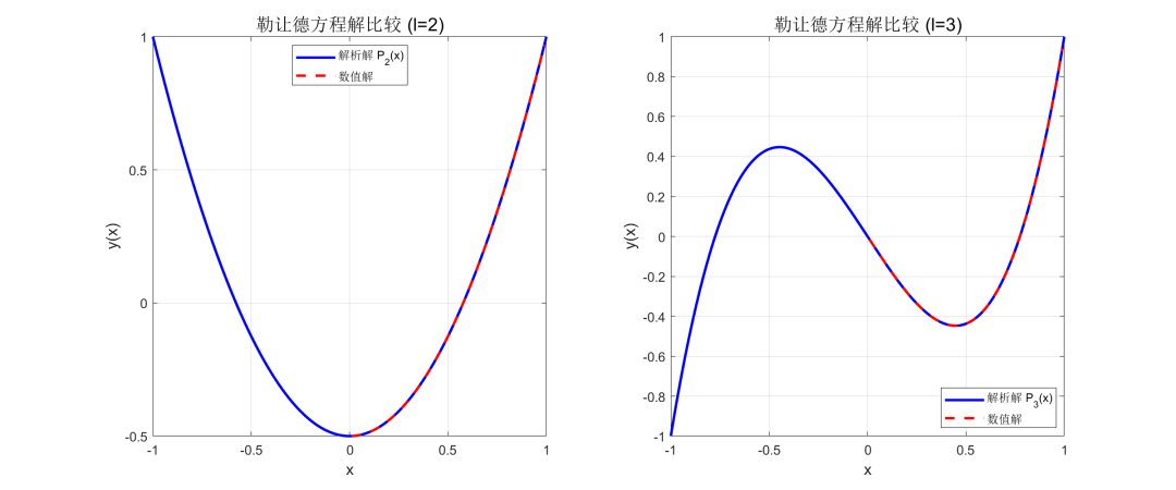
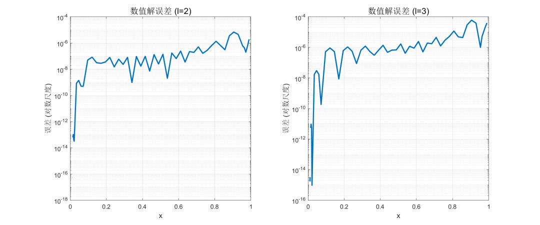
Conclusion: Through the power series method, we derived the polynomial solution of Legendre’s equation when the parameter is an integer—the Legendre polynomial. The comparison of numerical calculations with analytical solutions confirms the correctness of the derivation.
End
 Rotate S to the n-th power
Learn more information
Scan to follow the public account
Give a “recommendation” for the best view~