Sharing Cutting-Edge Research on TinyML
01
Definition
TinyML, or “Tiny Machine Learning,” refers to the technology, tools, and methodologies for running machine learning applications on ultra-low-power microcontrollers (MCUs) and other small computing devices. The core of TinyML is to compress and optimize trained machine learning models to fit the limited memory (typically KB-level SRAM, MB-level flash) and processing capabilities (usually simple CPUs with frequencies ranging from tens to hundreds of MHz, such as the Arm Cortex-M series, lacking powerful GPUs or NPUs) of these devices. This enables AI functionality to run locally at the source in the physical world (at the sensor end), rather than relying on the cloud or high-performance edge servers, while also ensuring low energy consumption and low cost. The reasons for developing TinyML are as follows:
Ultra-low power consumption: TinyML devices typically operate at milliwatt or even microwatt levels, aiming for months to years of continuous operation using button batteries or energy harvesting technologies.
Ultra-low latency: The inference process is completed directly on the local device, with response times reaching milliseconds, meeting the real-time requirements of applications such as industrial control and anomaly detection.
Low cost: The target hardware consists of very low-cost (usually a few dollars or even less) MCUs and sensors, making large-scale deployment feasible.
Adaptation to extremely low computing power: It can run stably on microcontrollers equipped with only simple CPUs and limited computing power, without relying on high-performance computing units.
02
Development Timeline
The development of TinyML can be divided into four key stages, each showing a gradual deepening in technological breakthroughs, hardware upgrades, and application implementations:
(1) Emergence Phase (Early 2010s and before)
Core Exploration: Academia and industry began to experiment with running simple pattern recognition algorithms on resource-constrained devices.
Technical Limitations: Deep Neural Networks (DNNs) were generally considered unsuitable for MCUs due to their computational and memory demands, limiting technological development to traditional simple algorithms.
(2) Technical Accumulation Phase (Mid to Late 2010s)
Model Compression Breakthrough: The deep learning community made significant progress in model compression techniques (such as quantization and pruning), proving that they could significantly reduce model size and accelerate inference, laying the core technological foundation for TinyML.
Initial Hardware Optimization: Prototypes of hardware accelerators for edge AI emerged, gradually improving the computational power and energy efficiency of MCUs, providing hardware support for subsequent model deployment.
(3) Explosion Phase (2018-2020)
Framework Support Implementation: The official release of TensorFlow Lite in 2019 marked the mainstream machine learning frameworks’ full support for MCU deployment, greatly lowering the development and application barriers for TinyML.
Emergence of Hardware Acceleration: Chip manufacturers began to launch dedicated MCUs for ultra-low-power AI inference, further promoting the popularization of TinyML technology through hardware-level computational and energy efficiency optimizations.
(4) Maturity and Deepening Application Phase (2021-Present)
Scaling of Technological Implementation: TinyML has transitioned from prototypes and pilot projects to large-scale commercial product deployments, with its cost-effectiveness and reliability validated in fields such as industrial IoT, consumer electronics, and smart buildings.
Explosion of Application Scenarios: Numerous application products have emerged, including industrial predictive maintenance, smart home sensors, wearable health monitoring, agricultural sensors, keyword wake-up, anomaly detection, and gesture recognition, with technology and industry becoming increasingly intertwined.
Improvement of Toolchains and Standards: Development toolchains have gradually matured, and the industry has begun to explore technical standards to further regulate the development and application of TinyML.
03
Core Mathematical Principles
The core mathematical principles of TinyML revolve around “model compression and optimization,” employing a series of technical means to reduce the number of model parameters and computational complexity, making them suitable for resource-constrained hardware (such as MCUs). The main techniques include model pruning, quantization, knowledge distillation, and neural architecture search:
(1) Model Pruning
1. Core Idea: Deep learning models contain a large number of redundant parameters. By removing “unimportant” weights (setting them to 0) in the weight matrix, computational resource consumption can be reduced and real-time performance improved while ensuring that model accuracy is minimally affected.
2. Algorithm Steps:
(1) Train the initial model normally to ensure it has basic performance;
(2) Prune the trained model by removing redundant weights or structures;
(3) Retrain the pruned model to recover accuracy lost due to pruning;
(4) Repeat the “train-prune-retrain” process until the model accuracy reaches the target threshold, then stop iterating.
3. Pruning Classification (by granularity and structure):
Unstructured Pruning: Pruning individual weights or neurons. A large number of weights can be removed without changing the overall network structure, but hardware acceleration is more challenging. Common methods include weight pruning and neuron pruning.
Structured Pruning: Pruning entire convolutional kernels, channels, or layers. The original convolution structure is preserved, making it easier to implement acceleration on hardware, but the pruning intensity is relatively limited. Common methods include filter pruning (e.g., based on L1 norm), channel pruning (e.g., based on BN layer scaling factors), group pruning, and stripe pruning.
(2) Model Quantization
1. Core Idea: Represent model parameters and computations with fewer bits, reducing model storage size, lowering memory usage, and accelerating inference. The core is to exchange a small loss in precision for a significant reduction in resource consumption.
2. Classification of Quantization Stages:
Post-training Quantization (PTQ): Offline quantization, where parameters are quantized after model training is complete, requiring no retraining. This is simple but may incur slightly higher accuracy loss.
Quantization-aware Training (QAT): Online quantization (pseudo-quantization), where quantization errors are simulated during training, allowing the model to adapt to the accuracy loss caused by quantization. The final quantized model has higher accuracy, but the training process is more complex.
3. Common Quantization Methods:
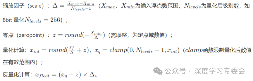
(1) Asymmetric Quantization
Applicable Scenario: When the input data distribution is asymmetric (e.g., activation values), zero-point shifting is needed to adapt to the data range.
Core Formula:
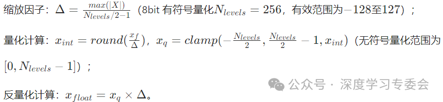
(2) Symmetric Quantization
Applicable Scenario: When the input data distribution is symmetric (e.g., weight values), the zero-point is fixed at 0, simplifying calculations.
Core Formula:
(3) Random Quantization
Similar to asymmetric quantization, but noise is introduced during the quantization process. The parameter calculation and de-quantization steps are consistent, suitable for noise-robust scenarios.
4. Common Quantization Strategies:
With hardware support, asymmetric quantization is applied to activation values (to adapt to asymmetric distributions), while symmetric quantization is applied to weight values (to simplify calculations), which is the mainstream solution balancing accuracy and efficiency.
(3) Knowledge Distillation (KD)
1. Core Idea: Transfer the “knowledge” of a large, complex model (Teacher Model) to a small, lightweight model (Student Model), allowing the student model to run on resource-constrained devices while maintaining performance close to that of the teacher model.
2. Knowledge Transfer Method:
Soft Labels: Compared to traditional hard labels (which only indicate categories), soft labels output by the teacher model contain relative probability distribution information between categories, providing richer learning signals for the student model.
Temperature Parameter (T): Controls the smoothness of the soft label distribution. A higher temperature results in a smoother distribution (providing more relative information between categories), while a lower temperature approaches hard labels. Adjusting T balances the effectiveness of knowledge transfer with the difficulty of model learning.
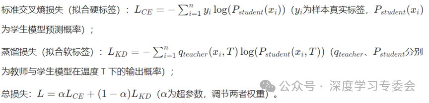
3. Loss Function Design:
The total loss is a weighted sum of the standard cross-entropy loss and the distillation loss, as shown in the formula below:
(4) Neural Architecture Search (NAS)
1. Core Idea: Use automated search algorithms to find the optimal neural network architecture within a predefined search space, optimizing targets such as accuracy, inference speed, and parameter count, reducing the cost and subjectivity of manual architecture design.
2. Three Key Elements:
1) Search Space: Defines all possible network structure components (such as convolutional layers, pooling layers, activation functions) and connection methods, determining the range and potential of the search.
2) Search Strategy: Algorithms that guide efficient exploration within the search space, balancing search efficiency and architecture performance. Common strategies include reinforcement learning-based, evolutionary algorithms, and gradient methods.
3) Performance Estimation: Quickly evaluates the performance of candidate architectures (e.g., through lightweight training, parameter sharing), avoiding full training for each architecture and improving search efficiency.
04
Algorithm Variants
(1) Algorithm Variant 1: AIfES (A Next-Generation Edge AI Framework)1. Core Objective: Address the limitations of traditional edge AI frameworks—low flexibility for target hardware and limited support for integrating custom hardware accelerators, bridging the gap between resource-constrained embedded systems and complex machine learning models.2. Core Features:Wide Hardware Adaptation: Supports all types of MCUs, from small 8-bit MCUs to high-performance ARM Cortex-M series MCUs, compatible with inference and device-side training for FCNN (Fully Connected Neural Networks) and CNNs.Modular Architecture: Composed of three main modules: ailayer (network layer), ailoss (loss function), and aiopti (optimizer), each containing a three-layer structure of “Type – Implementation – Data Type,” supporting flexible configurations (e.g., ailayer can choose dense_layer/conv2d_layer, implementation can choose default/CMSIS/RISC-V, and data types can support f32/q15/q7).3. Workflow:(1) Model Creation: Build a custom network structure based on the ailayer module by selecting the network layer type, implementation method, and data type;(2) Loss Selection: Determine the type of loss function (e.g., MSE, cross-entropy) through the ailoss module to adapt to task requirements;(3) Optimizer Selection: Configure the optimizer (e.g., SGD, ADAM) using the aiopti module to adjust the training process;(4) Model Training: Supports device-side training without relying on cloud computing power.4. Key Optimizations (Memory and Runtime):Memory Optimization:Supports automatic deletion of unused code to reduce code size;Separately allocates memory for ANN parameters and intermediate results to avoid memory waste;Provides a memory planner function to pre-calculate required memory and allocate it, with no internal dynamic memory allocation (except for stack-based local variables), ensuring system stability.Runtime Optimization:Includes startup functions and layers optimized for runtime, further improving efficiency except for matrix multiplication layers;Uses piecewise linear approximation (PLA) to optimize startup functions, trading slight precision loss for speed improvement;Does not perform automatic differentiation, providing two backpropagation workflows to reduce training memory consumption; supports model quantization to adapt to low-resource hardware.5. Performance Evaluation:Memory Consumption: At f32 and q7 precision levels, AIfES’s RAM and Flash consumption is lower than TensorFlow Lite Micro (TFLM), regardless of whether CMSIS acceleration is used, especially evident in complex networks (e.g., a 10×10 hidden layer network on the MNIST dataset);Execution Time: In FCDNN (Fully Connected Deep Neural Network) tests, AIfES (with CMSIS) has shorter execution times than TFLM (e.g., AIfES for FCDNN 1 is 8.67ms, TFLM is 9.69ms);Device-side Training: On the NRF52840 DK development board, training on the MNIST dataset takes only 1.19s per batch, with RAM usage at 104.14kB and Flash usage at 39.60kB, balancing efficiency and resource consumption.(2) Algorithm Variant 2: DERO (Deep Reorganization: Retaining Residuals in TinyML)1. Core Issue:Residual connections are key components of modern high-performance DNN models (e.g., ResNet, DenseNet), but they require additional memory buffers to store intermediate computation results, significantly increasing peak memory usage and making deployment on micro devices impossible:(1) Directly removing residual connections (“plain style” model): While this reduces memory, it results in significant accuracy loss (0.5%-11%);(2) Traditional memory optimization techniques (depth-first inference, operator reordering, etc.): Only optimize feature map memory usage and cannot eliminate the additional memory requirements of residual connections themselves.2. Core Solution: Two-step Optimization Strategy(1) Perception-based Residual ReconstructionObjective: Replan the starting and ending points of residual connections to eliminate additional memory buffers while ensuring effective gradient propagation (maintaining training efficiency).Key Observation:In-place Operation: Directly overwrites input memory to store output, requiring no additional memory;Non-in-place Operation: Requires new memory to store output, retaining input memory.Implementation Steps: ① Copy Skeleton: Copy the original model structure, removing all original residual connections to obtain a no-residual “skeleton” model; ② Select Residual Endpoint: Traverse model operations and insert residual aggregation points (new residual endpoints) before non-in-place operations (e.g., convolutions), using the input buffer of that operation to store aggregation results, eliminating the need for additional buffers; ③ Select Residual Starting Point: Use the previous residual endpoint as the next residual starting point to construct a continuous “residual chain,” ensuring smooth gradient propagation.(2) Residual-aware Operation OptimizationObjective: Address potential issues of tensor dimension mismatches and abnormal input feature distributions that may arise after residual reconstruction, ensuring effective model computation and accuracy.Implementation Steps: ① Hyperparameter Redistribution and Tensor Reshaping: Hyperparameter Redistribution: Calculate invalid parameters caused by residual changes and evenly distribute their “workload” across related operations; Tensor Reshaping: Use low-cost operations (1×1 point convolution to adjust channel numbers, pooling to reduce width and height, padding to increase width and height, BN layers to stabilize gradients) to adapt the dimensions of the main and branch feature maps of the new residual connections, ensuring normal computation. ② Input Normalization and Operation Fusion: Operation Reordering: Change the order from “Convolution (Conv) → Batch Normalization (BN) → ReLU” to “BN → ReLU → Conv,” allowing normalization to occur before convolution, enhancing training stability; Operation Fusion: Merge “BN → ReLU → Conv” into a single operation, absorbing the statistics and scaling/translation parameters of BN into the convolution weights and biases, reducing memory usage and accelerating inference.3. Performance Advantages:Memory Efficiency: The DERO reorganized model (DERO(P)) has memory efficiency comparable to the no-residual model (Plain(P)), with peak memory for ResNet50 reduced from 600KB in the original model to 120KB, and even more significant optimization for DenseNet121 (27% lower than Plain(P));Accuracy Retention: Effectively retains model accuracy while reducing memory, avoiding the accuracy loss caused by directly removing residual connections;Compatibility: Can be combined with depth-first inference (Patch-based) to further reduce memory consumption (26%-75% lower than the original model).(3) Algorithm Variant 3: Multi-modal Context-Aware Stress Recognition TinyML System1. Core Issues and Technical Bottlenecks:Traditional solutions are limited: Stress detection relies on cloud or large devices (e.g., smartphones), leading to high latency, privacy risks, and bulky devices;Hardware Constraints: MCUs have small memory (only 256KB) and weak computing power (ARM Cortex-M4), making it difficult to deploy complex models;Signal Interference: Heart rate (HR, based on PPG signals) and electrodermal activity (EDA) are easily affected by motion artifacts (e.g., signal distortion while walking).2. System Design: Dual-Model Collaborative Architecture(1) Model 1: Human Activity Recognition (HAR) ModelInput: Three-axis accelerometer data (built-in IMU sensor);Task: Real-time classification of user states (stationary: sitting/standing; moving: walking/running/climbing stairs);Performance: Binary classification accuracy of 98%, model size only 152KB, efficiently running on MCUs;Core Role: Serves as a context trigger condition, activating the stress detection model only when the user is detected to be stationary, avoiding interference from motion artifacts.(2) Model 2: Stress Detection ModelInput: Raw heart rate amplitude (PPG) and electrodermal activity (EDA) signals;Trigger Mechanism: Activated by the HAR model, running only in stationary states;Performance: Classification accuracy of 88%, model size after quantization compression is 1.1MB, fitting MCU resource constraints;Architecture Optimization: The optimal structure was determined through multiple rounds of variant testing (see Table 1).① CNN Architecture Variants (Number of Layers):In designing the stress detection model, the author explicitly tried different numbers of CNN layers:Initial Attempt (4-layer CNN): Used a CNN with four convolutional layers, achieving an accuracy of 95.6%.Performance and Resource Conflict: This 4-layer model occupied 97% of the dynamic memory of the Arduino Nano 33 Sense even after using int8 quantization, making it impossible to deploy alongside the activity recognition model.Simplified Variant (2-layer CNN): Reduced to two convolutional layers to meet memory constraints. This led to a 7.6% drop in accuracy (from 95.6% to 88%), but the model size was reduced by 67%, making it deployable.Further Simplification Attempt (1-layer CNN): Attempted to use only one convolutional layer to further reduce the model size. However, this caused a significant drop in accuracy to 61.8% (a decrease of 26.7%), which was an unacceptable sacrifice.Conclusion: The two-layer CNN structure was selected as the best variant for the stress detection model, achieving a balance between resource constraints and acceptable accuracy loss.② Quantization Strategy Variants:To adapt the model to extremely limited microcontroller resources, the author systematically tested different post-training quantization (PTQ) strategies.Specific Applications:HAR Model: Attempting int8 quantization led to excessive preprocessing complexity (due to the data range issues of the dataset), while float32 was too large. Ultimately, float16 quantization was chosen, with only a 0.34% loss in accuracy.Stress Detection Model: The model size after float16 quantization (92% storage usage) still could not meet the requirements for simultaneous deployment with the HAR model. The final choice was int8 quantization, reducing memory usage by 75% with no loss in accuracy.③ Algorithm Type Comparison (CNN vs. LSTM):When selecting models, LSTM was tested as an alternative algorithm variant to CNN, but compared to LSTM, CNN is lighter and has lower latency (stress model latency is 3642ms, HAR is only 26ms).④ Feature Engineering Variants (Stress Model):Initially explored using more features (e.g., BPM, HRV) to train the stress detection model.Models with these additional features became too large to deploy alongside the HAR model in the limited flash memory (1MB) of the microcontroller.The final stress model variant used only the raw HR amplitude and raw EDA values as input features. This is a simplification variant at the model input/feature level, driven by hardware constraints.3. System Advantages (Compared to Traditional Cloud Solutions)(1) Real-time response, suitable for latency-sensitive scenarios in healthcare;(2) Complies with medical data regulations, protecting user privacy;(3) Battery life of several days/weeks, suitable for wearable devices;(4) Suitable for large-scale deployment, especially in remote areas.4. Application ValueThrough the three core technologies of “micro hardware + quantized models + context triggering,” TinyML has demonstrated its advantages in low power consumption, privacy protection, and real-time performance, providing a complete paradigm of “edge intelligence – multi-model collaboration” for medical wearable devices, promoting the implementation of edge intelligence in health monitoring.
05
Applications and Implementations
(1) Core Application Areas
TinyML, with its low power consumption, low cost, and low latency characteristics, has achieved large-scale applications in various fields, with core scenarios including:
1. Predictive Maintenance
① Core Value: Real-time monitoring of machine performance characteristics, providing early warnings and triggering maintenance before failures occur, reducing downtime and repair costs, and enhancing production efficiency and safety.
② Application Case: A mining company deployed TinyML devices on rail cars to monitor the risk of wheel, bearing, and axle failures. A certain company identified issues a week in advance using this technology, reducing maintenance events by 50% over five years and saving approximately $34 million.
2. Smart Agriculture
① Core Value: Optimize agricultural production processes based on real-time environmental data and crop status analysis, increasing crop yields and reducing resource consumption (e.g., water and fertilizer).
② Typical Applications:
Crop Pest and Disease Monitoring: Deploy CNN models on edge devices, combined with drones for real-time identification of crop diseases;
Soil Quality Monitoring: Use TinyML models to analyze soil moisture and nutrient content in real-time, optimizing irrigation and fertilization strategies;
Livestock Health Monitoring: Analyze individual livestock behavior and physiological data to assess health status in real-time, reducing disease risks.
3. Smart Cities
① Core Value: Achieve refined management of urban environments, traffic, and safety through distributed micro-intelligent devices, enhancing urban operational efficiency and residents’ quality of life.
② Typical Applications:
Smart Security: Deploy TinyML models in homes and public areas for intrusion detection and abnormal behavior recognition;
Environmental Monitoring: Real-time monitoring of air quality, noise, and temperature/humidity, providing data support for urban environmental governance;
Smart Traffic: Integrate TinyML models into traffic monitoring devices for real-time analysis of traffic flow, optimizing traffic signal scheduling.
4. Healthcare
① Core Value: Achieve decentralization and portability of medical monitoring and diagnosis, reducing medical costs and improving service accessibility (especially in remote areas).
② Typical Applications:
Real-time Health Monitoring: Deploy TinyML models on wearable devices to monitor heart rate, blood pressure, ECG (electrocardiogram) abnormalities, and non-invasive blood glucose levels;
Medical Assistance: For example, gesture recognition models on surgical equipment to assist doctors in performing precise operations;
On-demand Diagnosis: Provide low-cost diagnostic solutions for resource-scarce areas, such as basic disease screening based on micro-devices.
5. Drones (UAVs) and the Internet of Things (IoT)
① Drone Applications:
Path Planning and Navigation: Use TinyML models to optimize flight paths in real-time, reducing energy consumption;
Environmental Monitoring: Equip micro-intelligent devices to detect road damage, forest fires, air quality, etc.;
Task Optimization: Dynamically allocate drone tasks to enhance multi-drone collaboration efficiency.
② IoT Applications:
Localized Data Processing: Perform real-time analysis of sensor data on IoT devices, reducing reliance on cloud services;
Energy Management: Optimize device energy consumption to extend battery life;
Security and Privacy: Process sensitive data locally to reduce the risk of privacy breaches during transmission.
(2) Key Software Frameworks and Platforms
The development and deployment of TinyML rely on dedicated frameworks and platforms, with the following being three mainstream tools:
1. TensorFlow Lite Micro:
TensorFlow is Google’s open-source lightweight machine learning framework that helps users quickly build deep learning computations in low-power, small hardware environments. TensorFlow Lite Micro is a lightweight AI engine for AIOT, designed to run machine learning models on microcontrollers and other resource-constrained devices. The edge-cloud link starts with TencentOS Tiny.
TensorFlow Lite Micro can easily compress regular TensorFlow models to just a few KB and comes with a large number of example models, such as Hello World or Magic Wand, to demonstrate various TinyML fundamentals and functionalities.
Invocation Method: Download the TensorFlow Lite Micro library from GitHub and follow the official documentation for model conversion and deployment.
2. Edge Impulse:
Edge Impulse is a platform specifically designed for developing TinyML applications. With its easy-to-use web-based interface, Edge Impulse is arguably the simplest solution for anyone to collect data, train models, and ultimately deploy them to microcontrollers.
Using Edge Impulse for TinyML development can leverage their Edge Optimized Neural (EON) compiler, which can run neural networks with 25-55% reduced memory and 35% reduced storage space compared to TFLite for microcontrollers. Like TFLite Micro, Edge Impulse supports a wide range of microcontrollers and development boards, including Arduino Nano 33 BLE Sense and Wio Terminal. Supported devices can easily record and upload datasets in minutes.
Invocation Method: Register on the Edge Impulse platform, upload data, train models, and deploy them to target devices using the provided SDK.
3. OpenMV:
OpenMV is another TinyML development platform focused primarily on computer vision applications. This includes machine learning applied to any type of image or video, such as object recognition or image classification. The platform is built around the OpenMV Cam H7, a microcontroller board running on the ARM Cortex M7 processor and is programmable in Micropython.
Additionally, OpenMV provides a cross-platform IDE with a powerful code editor, debugging terminal, and frame buffer viewer with histogram display—all key components for developing computer vision applications in TinyML.
Invocation Method: Upload models to OpenMV hardware via the OpenMV IDE, and configure and run them.
Editorial Team
Writers: Chen Weiling, Fu Xinrui, Wang Yujing, Lu Qiuting
Editors: Chen Weiling
Final Review: Zhao Tiesong, Xu Long