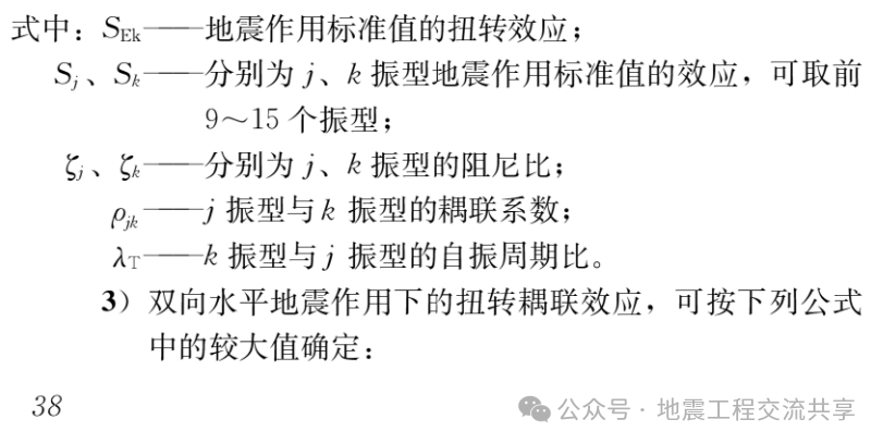
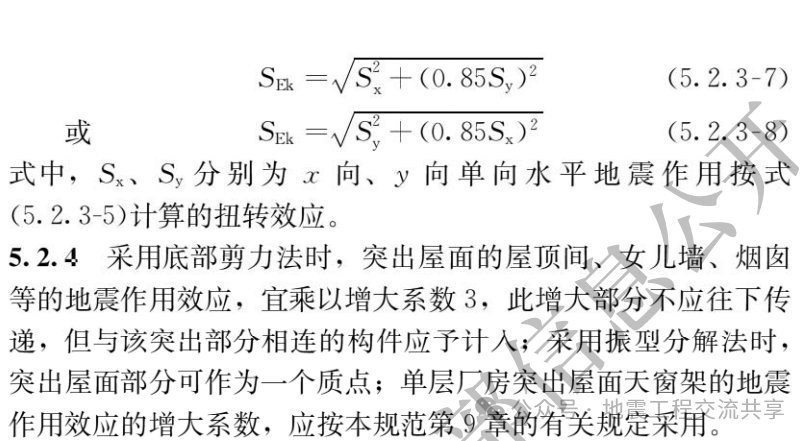
The “Code for Seismic Design of Buildings” GB50011-2016, Section 5.2.2: When using the modal decomposition response spectrum method…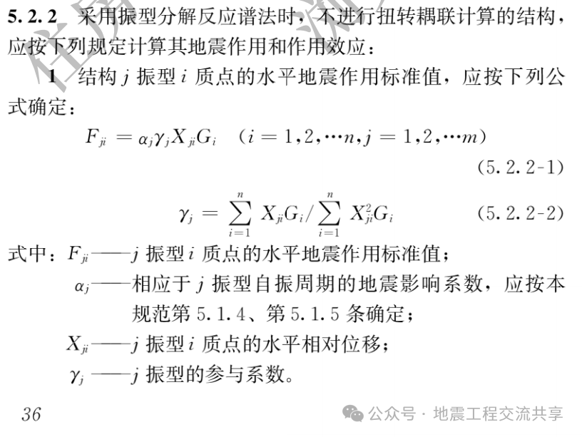
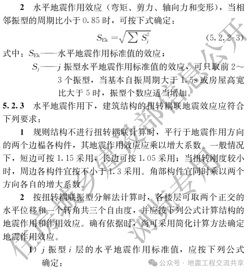
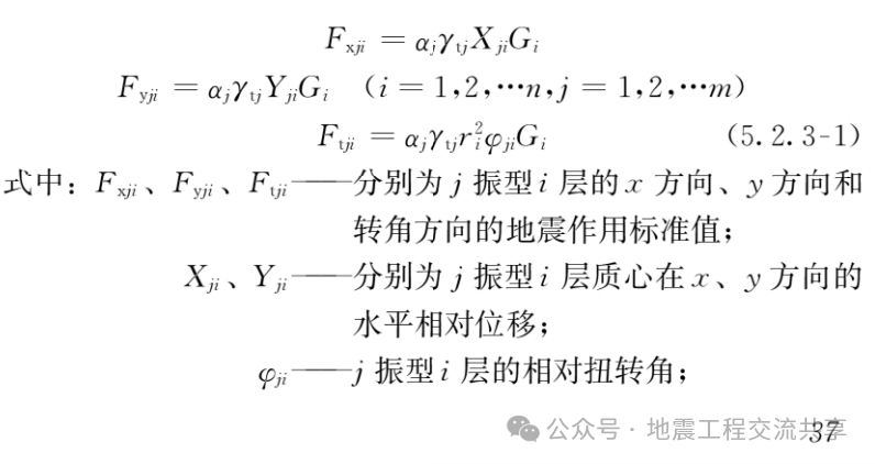
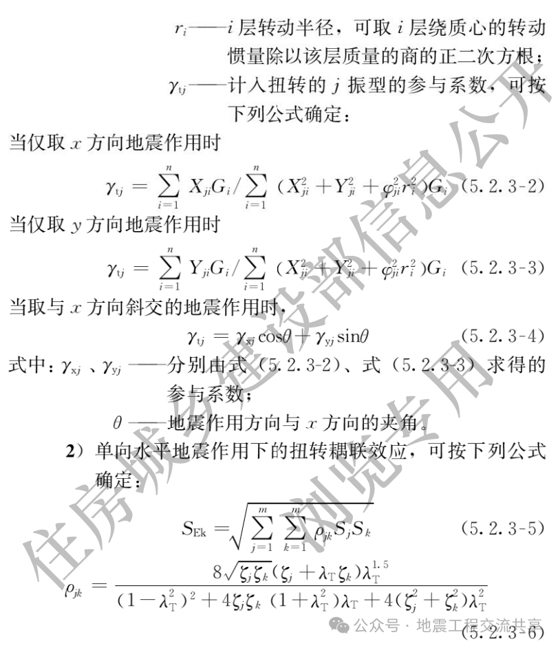
 Advantages and Disadvantages:
The modal decomposition response spectrum method, in simple terms, imagines a multi-story building as several “independent pendulums,” each corresponding to a natural vibration period and mode shape. First, the maximum seismic force for each pendulum is calculated, and then the peak values of each mode shape are combined using SRSS or CQC to obtain the internal forces and displacement envelope of the entire building. Its strengths and weaknesses are concentrated in this approach.
Advantages:
Intuitive concept: Period—Mode shape—Spectrum value—Combination, a straightforward line that makes it easy for designers to grasp.
Fast calculations: Only one eigenvalue problem needs to be solved, and by referencing the code spectrum curve, results for high-rise buildings can be obtained in minutes.
Seamless integration with codes: The spectrum can be directly switched for small, medium, and large earthquakes without needing to reselect the wave.
Stable results: Differences in comparisons of different schemes for the same model are controllable, facilitating scheme optimization.
Accurate in the elastic stage: Differences under small earthquakes and wind-induced vibrations are usually controlled within 5% compared to time history analysis.
Disadvantages:
Linear only: Material yielding, stiffness degradation, and energy dissipation from dampers cannot be included, leading to an overestimation of safety under large earthquakes.
Higher mode shapes may be missed: When the aspect ratio is large or there is a whip effect at the top, using only the first 3-6 modes may underestimate the upper displacement.
Combination rules have errors: When periods are dense or torsional coupling is severe, CQC may still differ by 10%-20%.
Does not provide time history: Only peak values can be obtained, and it cannot show how shear forces change over time, nor can it depict hysteretic energy dissipation.
Not friendly to irregular structures: Planar concavities, abrupt changes in vertical stiffness, isolation layers, and energy-dissipating supports require additional analysis.
Poor site specificity: A single spectrum represents an average earthquake, and cannot reflect near-fault pulses or long-period seismic motions.
In summary: Small earthquakes require computational power, while large earthquakes require fate—this method is sufficient for conventional high-rises, but for extreme cases, isolation, or large spans, time history or pushover analysis must be supplemented.
MATLAB calculations are as follows:
Structural dynamic characteristics:
1st mode: Period = 0.181s, Frequency = 5.515Hz, Participation factor = 12.623
2nd mode: Period = 0.264s, Frequency = 3.788Hz, Participation factor = 33.895
3rd mode: Period = 0.819s, Frequency = 1.220Hz, Participation factor = -140.327
Inter-story shear force results:
1st floor: Shear force = 16.29kN
2nd floor: Shear force = 9.62kN
3rd floor: Shear force = 4.28kN
Show mode shape superposition animation? (1=yes, 0=no): 1
MATLAB plots are as follows: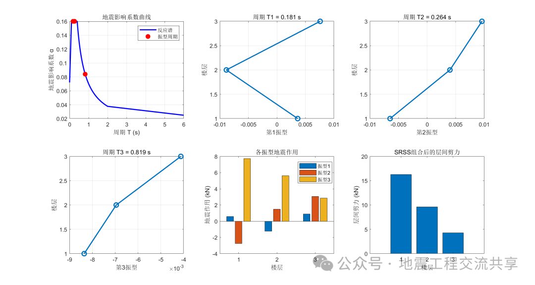
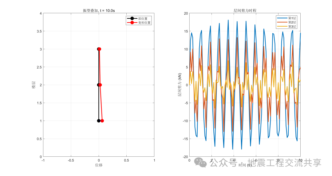 MATLAB code is as follows:
%% Modal Decomposition Response Spectrum Method Visualization
% "Code for Seismic Design of Buildings" (GB 50011-2016)

clear; clc; close all;

%% Parameter settings
% Structural parameters
m = [8000, 7000, 6000]';  % Mass of each floor (kg)
k = [2.8e6, 2.4e6, 2.0e6]';    % Stiffness of each floor (N/m)
n = length(m);          % Number of floors
h = [4.0, 3.5, 3.5]';   % Floor height (m)

% Seismic parameters
Tg = 0.40;              % Characteristic period (s) - Design earthquake group first group, site category II
alpha_max = 0.16;       % Maximum horizontal seismic impact coefficient - 7 degrees 0.1 g
zeta = 0.05;            % Damping ratio

%% 1. Calculate frequency and mode shapes
% Construct mass matrix and stiffness matrix
M = diag(m);
K = zeros(n);

% Correctly construct the stiffness matrix (tridiagonal matrix)
for i = 1:n
    if i == 1
        K(i,i) = k(i);
        if n > 1
            K(i,i+1) = -k(i);
        end
    elseif i == n
        K(i,i) = k(i-1) + k(i);
        K(i,i-1) = -k(i-1);
    else
        K(i,i) = k(i-1) + k(i);
        K(i,i-1) = -k(i-1);
        K(i,i+1) = -k(i);
    end
end

% Solve eigenvalue problem
[V, D] = eig(K, M);
omega = sqrt(diag(D));          % Circular frequency
T = 2*pi./omega;                % Period

% Sort by period
[T, idx] = sort(T);
V = V(:, idx);
omega = omega(idx);

%% 2. Calculate seismic impact coefficient curve
T_range = linspace(0, 6, 600);  % Extend period range to 6s
alpha = zeros(size(T_range));

% Calculate seismic impact coefficient according to code 5.1.5
for i = 1:length(T_range)
    Ti = T_range(i);
    if Ti < 0.1
        alpha(i) = (0.45 + 5.5*Ti) * alpha_max;
    elseif Ti < Tg
        alpha(i) = alpha_max;
    elseif Ti < 5*Tg
        alpha(i) = (Tg/Ti)^0.9 * alpha_max;
    elseif Ti <= 6
        alpha(i) = (0.2^0.9 - 0.02*(Ti-5*Tg)) * alpha_max;
    else
        alpha(i) = 0;
    end
end

%% 3. Modal decomposition calculation
% Calculate participation factors for each mode
Gamma = zeros(n,1);
for j = 1:n
    Gamma(j) = (V(:,j)' * M * ones(n,1)) / (V(:,j)' * M * V(:,j));
end

% Calculate seismic actions for each mode
F = zeros(n,n);
for j = 1:n
    % Find corresponding seismic impact coefficient
    if T(j) <= 6
        % Directly calculate seismic impact coefficient to avoid using interp1
        if T(j) < 0.1
            alpha_j = (0.45 + 5.5*T(j)) * alpha_max;
        elseif T(j) < Tg
            alpha_j = alpha_max;
        elseif T(j) < 5*Tg
            alpha_j = (Tg/T(j))^0.9 * alpha_max;
        else
            alpha_j = (0.2^0.9 - 0.02*(T(j)-5*Tg)) * alpha_max;
        end

        % Calculate mode seismic action (F_j = α_j * γ_j * X_j * G_i)
        F(:,j) = alpha_j * Gamma(j) * V(:,j) .* (m * 9.8);
    else
        % Period greater than 6s, seismic impact coefficient is 0
        F(:,j) = zeros(n,1);
    end
end

%% 4. Combine responses of each mode (SRSS method)
% Calculate inter-story shear forces for each mode
V_shear = zeros(n,n);
for j = 1:n
    % Calculate shear forces from top to bottom
    V_shear(:,j) = flipud(cumsum(flipud(F(:,j))));
end

% SRSS combination
V_total = sqrt(sum(V_shear.^2, 2));

%% 5. Visualize results
figure('Position', [100, 100, 1200, 800]);

% Subplot 1: Seismic impact coefficient curve
subplot(2,3,1);
plot(T_range, alpha, 'b-', 'LineWidth', 2);
hold on;
for j = 1:min(3,n)
    if T(j) <= 6
        % Directly calculate seismic impact coefficient
        if T(j) < 0.1
            alpha_j = (0.45 + 5.5*T(j)) * alpha_max;
        elseif T(j) < Tg
            alpha_j = alpha_max;
        elseif T(j) < 5*Tg
            alpha_j = (Tg/T(j))^0.9 * alpha_max;
        else
            alpha_j = (0.2^0.9 - 0.02*(T(j)-5*Tg)) * alpha_max;
        end
        plot(T(j), alpha_j, 'ro', 'MarkerSize', 8, 'MarkerFaceColor', 'r');
    end
end
xlabel('Period T (s)');
ylabel('Seismic impact coefficient α');
title('Seismic impact coefficient curve');
grid on;
legend('Response spectrum', 'Mode period');

% Subplots 2-4: Mode shapes
for j = 1:min(3,n)
    subplot(2,3,1+j);
    plot(V(:,j), 1:n, 'o-', 'LineWidth', 2, 'MarkerSize', 8);
    xlabel(['Mode ', num2str(j)]);
    ylabel('Floor');
title(['Period T', num2str(j), ' = ', num2str(T(j), '%.3f'), ' s']);
grid on;
end

% Subplot 5: Seismic actions for each mode
subplot(2,3,5);
bar(F/1000); % Convert to kN
xlabel('Floor');
ylabel('Seismic action (kN)');
title('Seismic actions for each mode');
legend_str = arrayfun(@(x) sprintf('Mode%d', x), 1:n, 'UniformOutput', false);
legend(legend_str, 'Location', 'best');
set(gca, 'XTick', 1:n);
set(gca, 'XTickLabel', 1:n);

% Subplot 6: Inter-story shear forces after combination
subplot(2,3,6);
bar(V_total/1000); % Convert to kN
xlabel('Floor');
ylabel('Inter-story shear force (kN)');
title('Inter-story shear forces after SRSS combination');
set(gca, 'XTick', 1:n);
set(gca, 'XTickLabel', 1:n);

%% 6. Output results
fprintf('Structural dynamic characteristics:\n');
for j = 1:n
    fprintf('Mode %d: Period=%.3fs, Frequency=%.3fHz, Participation factor=%.3f\n', ...
        j, T(j), omega(j)/(2*pi), Gamma(j));
end

fprintf('\nInter-story shear force results:\n');
for i = 1:n
    fprintf('Floor %d: Shear force=%.2fkN\n', i, V_total(i)/1000);
end

%% 7. Animate mode shape superposition
animate = input('Show mode shape superposition animation? (1=yes, 0=no): ');
if animate == 1
    figure('Position', [200, 200, 1000, 600]);

    % Set animation parameters
    t_max = 10; % Maximum time
    dt = 0.1;   % Time step
    scale = 0.5; % Displacement scaling factor

    % Pre-calculate time history
    time_points = 0:dt:t_max;
    time_history = zeros(n, length(time_points));

    for idx = 1:length(time_points)
        t = time_points(idx);

        % Calculate displacements for each mode
        total_disp = zeros(n,1);
        for j = 1:n
            if T(j) <= 6
                % Directly calculate seismic impact coefficient
                if T(j) < 0.1
                    alpha_j = (0.45 + 5.5*T(j)) * alpha_max;
                elseif T(j) < Tg
                    alpha_j = alpha_max;
                elseif T(j) < 5*Tg
                    alpha_j = (Tg/T(j))^0.9 * alpha_max;
                else
                    alpha_j = (0.2^0.9 - 0.02*(T(j)-5*Tg)) * alpha_max;
                end

                total_disp = total_disp + V(:,j) * sin(omega(j)*t) * Gamma(j) * alpha_j;
            end
        end

        % Calculate inter-story shear forces at current time
        V_current = zeros(n,1);
        for j = 1:n
            if T(j) <= 6
                % Directly calculate seismic impact coefficient
                if T(j) < 0.1
                    alpha_j = (0.45 + 5.5*T(j)) * alpha_max;
                elseif T(j) < Tg
                    alpha_j = alpha_max;
                elseif T(j) < 5*Tg
                    alpha_j = (Tg/T(j))^0.9 * alpha_max;
                else
                    alpha_j = (0.2^0.9 - 0.02*(T(j)-5*Tg)) * alpha_max;
                end

                F_current = alpha_j * Gamma(j) * V(:,j) .* (m * 9.8) * sin(omega(j)*t);
                V_current = V_current + flipud(cumsum(flipud(F_current)));
            end
        end

        time_history(:, idx) = V_current/1000; % Convert to kN

        % Plot structural deformation
        subplot(1,2,1);
        cla;
        plot(zeros(n,1), 1:n, 'k-o', 'LineWidth', 2, 'MarkerSize', 8, 'MarkerFaceColor', 'k');
        hold on;
        plot(total_disp*scale, 1:n, 'r-o', 'LineWidth', 2, 'MarkerSize', 8, 'MarkerFaceColor', 'r');

        for i = 1:n
            plot([0, total_disp(i)*scale], [i, i], 'b--');
        end

        xlim([-1, 1]);
        ylim([0, n+1]);
        xlabel('Displacement');
        ylabel('Floor');
        title(['Mode shape superposition, t = ', num2str(t, '%.1f'), 's']);
        grid on;
        legend('Original position', 'Deformed position');

        % Plot inter-story shear force time history
        subplot(1,2,2);
        plot(time_points(1:idx), time_history(:, 1:idx)', 'LineWidth', 2);
        xlim([0, t_max]);
        xlabel('Time (s)');
        ylabel('Inter-story shear force (kN)');
        title('Inter-story shear force time history');
        grid on;
        legend_str = arrayfun(@(x) sprintf('Floor %d', x), 1:n, 'UniformOutput', false);
        legend(legend_str, 'Location', 'best');

        drawnow;
    end
end