MATLAB Image Processing | Logarithmic Transformation Code Design (Complete Code Included)

The logarithmic transformation changes the brightness distribution of an image by taking the logarithm of the gray value of each pixel, which is a common method for image gray level transformation.

The logarithmic transformation can improve imaging quality under uneven lighting conditions and also adjust high dynamic range data.

The following provides example code for logarithmic transformation, including functions for setting appropriate display parameters.

Additionally, it demonstrates the use of <span>tiledlayout</span> to replace <span>subplot</span> for subplot display, high-quality curve plotting, and LaTeX display of variables.

Example 3-1-3 Implement the logarithmic transformation of the input grayscale image, displaying both the original image and the transformed result. The specific implementation code is as follows.

%=========================================================================
% DEMO: Logarithmic Transformation for Image
%    Name: IMLOG
%    IDIPLAB, 
%    School of Information and communication engineering,
%    University of Electronic Science and Technology of China
%    Date: 2025.09.09; revised 
%    Author：Zhenming Peng
%
% See Also IMADJUST, STRCTCHLIM, BRIGHEN
%=========================================================================
clc, clear, close all;

I = imread('data\perroquet.png'); % Read an image

t = tiledlayout(1,2);  % Create tiled chart layout for displaying subplots

nexttile,              % subplot(121)
imshow(I)

title('The Original Image','FontSize',12)

if ndims(I)==3          
   I = rgb2gray(I);    % Convert to grayscale image
end

if ~isa(I,'double')
     I = double(I);    % Convert to double image
end

c = 1.8;
lg = c*(log(I+1));

%=========================================================================
lg = mat2gray(lg);               % Intensity [0 1]
% lg = im2uint8(mat2gray(lg));   % [0 255]
% lg = (lg-abs(min(lg(:))))./(max(lg(:))-min(lg(:))); % Intensity [0 1]
% lg = uint8(mat2gray(lg)*255);  % [0 255]

nexttile,                        % subplot(122), 
imshow(lg,[]); title('The Log Image','FontSize',12)
t.TileSpacing = 'tight';         % 'loose','compact','tight','none'
t.Padding = 'compact';           % 'loose','compact','tight'

set(gcf,'Color','White');        % White Background


%=========================================================================
r = 0:1:255;
s = c.*log(1+r);
%==========================================================================

figure,
MarkerPoints = ceil(linspace(1,length(s),5));
plot(r,s,'r-o','LineWidth',2.0, ...
    'MarkerIndices',MarkerPoints,...
    'MarkerSize',10,...
    'MarkerFaceColor',[0,1,0]);
title('Log transform curve')
xlabel('$f(x,y)$','Interpreter','latex');
ylabel('$g(x,y)$','Interpreter','latex');
xlim([0,255]),ylim([min(s),1.02*max(s)]);

annotation('arrow',[0.54 0.39],[0.64 0.75],'Color','b','LineWidth',1.2);
text(120,5.8,'$g(x,y)=clog(1+f(x,y))$',...
    'Interpreter','latex','FontSize',14);

% hold on; box on

% Figure decoration
defaultAxes

% Enlarge figure with specified size and position
set(gcf,'Units','Normalized', 'OuterPosition', [0.35 0.12 0.30 0.45]);

% White Background
set(gcf,'Color','w'); 

The program output is as follows:

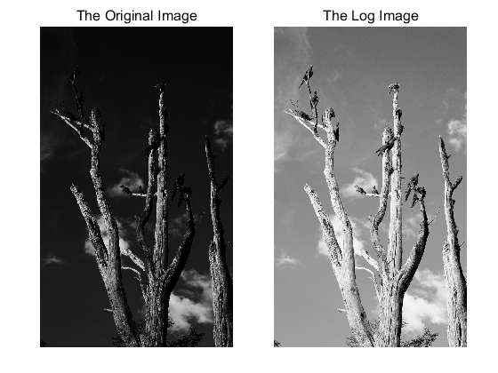Figure 1 Comparison of results before and after transformation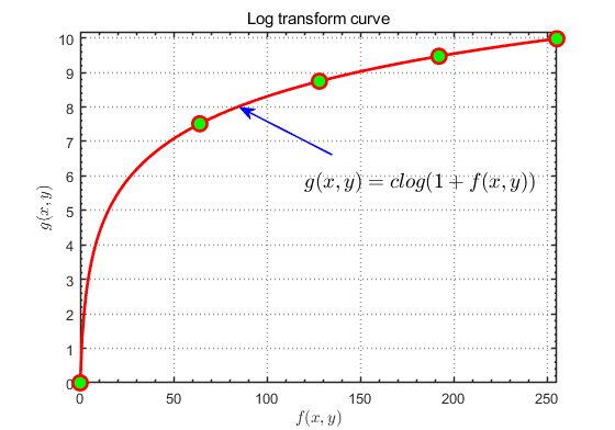Figure 1 Logarithmic transformation curve

Editor’s note: This post has no commercial purpose and is only for teaching and technical sharing. Some reference codes are provided with sources. If there is any infringement, it will be deleted immediately.

“To understand why I couldn’t sleep yesterday, I couldn’t sleep again today.”

Image and text: Zhenming Peng

Editor: Simin LiuPreviousIssuesReview

MATLAB Image Processing | Constructing Frequency Domain Filters from Spatial Domain Templates (Complete Code Included)

MATLAB Plotting Techniques | Setting Transparency of Color Bars (Complete Code Included)

MATLAB Plotting Techniques | Capturing Frames to Generate GIF Animations (Complete Code Included)

MATLAB Plotting Techniques | Standard Labeling of Graphics (With Example Code)

MATLAB Signal Simulation | Understanding Frequency Resolution of Fourier Transform (With Example Code)

MATLAB Image Processing | Homomorphic Filtering of Grayscale Images (Complete Code Included)

MATLAB Plotting Techniques | Drawing Dual Y-Axis Line Charts (With Example Code)

MATLAB Image Processing | Sigmoid Function Contrast Stretching (With Example Code)

MATLAB Plotting Techniques | Gamma Transformation Curve of Grayscale Images (With Example Code)

MATLAB Plotting Techniques | Clever Use of Graphics Handles (With Example Code)

MATLAB Plotting Techniques | Area Filling Between Two Lines with Color (With Source Code)

MATLAB Plotting Techniques | Optimization of 3D Visualization Code for Fourier Series Expansion

MATLAB Plotting Techniques | Data Visualization Color Schemes (With Code)

MATLAB Plotting Techniques | Pseudocolorization of Grayscale Images (With Code)

MATLAB Plotting Techniques | Density Scatter Plot + Regression without Solid Lines (With Code)

MATLAB Plotting Techniques | 2D Scatter Plot (With Code)

MATLAB Plotting Techniques | 3D Curve Filling (With Code)

MATLAB Plotting Techniques | 3D Line Chart (With Code)

MATLAB Plotting Techniques | 3D Surface (With Code)

MATLAB Plotting Techniques | Homemade Music Player (With Code)

MATLAB Plotting Techniques | Polygon Area Filling Chart (With Code)

MATLAB Plotting Techniques | Drawing Color Gradient Line Charts (With Code)

MATLAB Plotting Techniques | Line Chart Drawing (With Code)

MATLAB Plotting Techniques | Color Gradient Bar Chart Drawing

What moves you is not someone else’s story, but the shadow of yourself read from someone else’s story.