Matlab Introduction Tutorial | 008 2D Plotting: Understanding Plot Usage

Author: Daniel

Date: 2020/8/24

Problem-oriented, starting from scratch, quick start, efficient learning, and mastering Matlab programming.

2D plotting is the foundation for all other types of plotting. We will introduce the details of 2D plotting in three articles!

Key Points of This Article

• Vectors and Matrices
• Array Operations
• Three Steps of Plotting

Mechanism of Matlab Plotting

Recalling the steps of drawing function graphs in high school helps us understand the plotting principles of Matlab. For example, to draw the graph of a function, we would do the following:

1. List:

2. Group points:

3. Plot points and connect them with a smooth curve to get a rough sketch of the curve.

Using Matlab to plot the graph of a single-variable function is similar to the above steps. Due to the powerful computing capabilities of computers, we only need to provide several values of the independent variable (mathematically known as a vector or one-dimensional array) and the function expression, and Matlab will automatically calculate the vector of function values. Additionally, the coordinate system is also generated automatically.

There are also three steps to plot using Matlab:

1. Provide the array of independent variables
2. Provide the expression for calculating the array of function values
3. Plot points and connect them with line segments

For example, if we want to plot a graph in Matlab with the independent variable array, it is not difficult to calculate the function value array. Open Matlab and write the following three lines in the command window to plot the “graph” of the function.

x=[-2 -1 0 1 2];
y=[4 1 0 1 4];
plot(x,y)

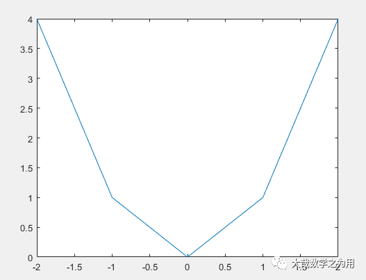
This graph looks like a clumsy “ugly duckling”, rough and ugly, far from the image we want! But don’t forget, the ugly duckling’s parents are white swans! We have a way to quickly improve and get the image we want!

Here, we want to illustrate two important things through this rough graph:

Principles of Matlab Plotting

1. Calculations in Matlab plotting are based on arrays;
2. Connections between points are made with line segments, technically known as “linear interpolation”;
3. When there are enough points (as long as the length of the vector, i.e., the number of components it contains, is long enough), the plotted graph will undergo a qualitative change, appearing continuous instead of discrete, and the polygon will appear as a smooth curve.

From a dialectical perspective, discreteness and continuity are opposites that are unified and can transform into each other. In fact, continuity is a concept that exists in thought, and in reality, we deal with and describe continuity through discreteness. The underlying idea is simple: points become lines, and when the spatial distance between points is close enough, they appear continuous.

The continuous curves we see on the computer are actually composed of sufficiently close discrete points (pixels). Our eyes are deceived, or we cannot distinguish the gaps between these points on the curve, leading us to feel that it is a continuous curve.

Mastering Plotting with the Three-Step Method

With just three simple commands, we can plot a decent graph, formatted as:

x=array;
y=array;
plot(x,y)

Having clarified the principles and steps of plotting, let’s improve the graph. We add 9 additional points in the closed interval with a step size of 0.4, expressed as the array x=[-2 -1.6 -1.2 -0.8 -0.4 0 0.4 0.8 1.2 1.6 2], thus including a total of 11 points at the interval endpoints.

Writing vectors like this can be cumbersome, but Matlab provides a smarter way to write it. Since the components of the vector form an arithmetic sequence with a common difference (or “step size”) of 0.4, Matlab offers two ways to describe the arithmetic sequence array:

1. Using a colon: formatted as x=start:step:end;
2. Using the linspace function: formatted as x=(start,end,number of points)

Thus, the vector with 11 components can be written as: x=-2:0.4:2 or: x=linspace(-2,2,11).

Now, to write the vector, we can utilize the operations and functions defined in Matlab to calculate the vector; we only need to provide the expression. You might already understand how to write the code, so let’s see if the following works:

x=linspace(-2,2,11);
y=x^2;
plot(x,y)

Press Enter and see what happens? An error appears:

Error using ^

Incorrect dimensions for raising a matrix to a power.

Check that the matrix is square and the power is a scalar.

To perform elementwise matrix powers,

use ‘.^’.

How did this happen? Beginners often fall into elementary mathematical thinking, naively believing that y=x^2 is correct. If it were a variable, this would represent a calculation. However, here it is an array, and we need to square each of its components, i.e.,

Matlab strictly distinguishes between numerical operations and array operations; array operations require a dot before the operator. Therefore, the expression should be written as: y=x.^2.

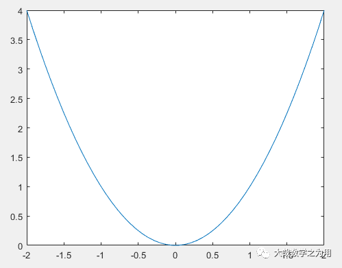
Running the following code will produce the correct graph:

x=-2:0.4:2;
y=x.^2;
plot(x,y)

The output graph looks much better now, but it’s still not ideal. Let’s reduce the step size a little:

x=-2:0.08:2;
y=x.^2;
plot(x,y)

This time, the plotted graph appears smoother:

Now let’s give an example of a trigonometric function: plotting the sine function on a closed interval.

This time, we take 101 points (including endpoints 0 and 2π). If we use a colon to write the independent variable array, we need to calculate the step size:

Generally, taking points uniformly on a closed interval (including both endpoints) is equivalent to dividing it evenly, so the formula for the step size is.

Thus, the code to plot the graph is as follows:

x=0:0.02*pi:2*pi;
y=sin(x);
plot(x,y)

Alternatively, we should use the linspace function to write the array more conveniently:

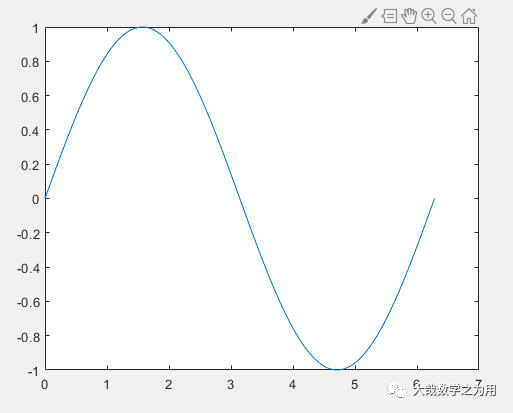
x=linspace(0,2*pi,101);
y=sin(x);
plot(x,y)

Here, for convenience in calculating the step size, we took 101 points. In reality, taking one less point does not significantly affect the result, so generally, when writing code with linspace, the number of points is often rounded to the nearest hundred for aesthetic reasons: x=(0,2*pi,100).

Running the above code, the resulting graph is as follows:

Have you learned the usage of plot? We can extend this to practice plotting five basic elementary functions: power functions, exponential functions, logarithmic functions, trigonometric and inverse trigonometric functions.

As a practice, try plotting the following function graphs:

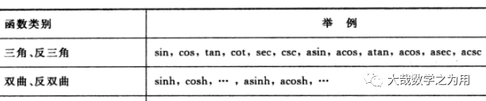
Note: The function expressions in Matlab differ from mathematical expressions (as mentioned above regarding array operation expressions), so we should not write them naively; it is best to consult books frequently. Here we provide the common function expressions in Matlab: